Hello all,
I've got a problem with a table I set up.
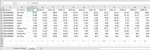
Here is the reference table:
And on another tab, I have this information in multiple tables for quarters of the year (I have 4 tables for each FY):
As you can see, in column B of the 2nd table, it includes a text string that contains both the Division # (as it shows in the first table), a "/", and then the employee number. What I need to do is to look up the division OH rate based on the Division # in the text string. I currently have a VLOOKUP using a LEFT formula in the Division OH Rate column in the second table, but now I need to add a column to the left of column C in the first table so I can enter the new year for the new year's quarters and it throws off every year because it's doing a VLOOKUP to the 3rd row or 4th row instead of doing a lookup by the actual year (I don't want to have to update each prior quarter's "col reference" each time I add a new year, in other words.
What I want to do is, in the 2nd table, column F (Division OH Rate) to look up the YEAR I listed in bold in cell A1 of the second table, plus look up the left side of the text string in column B of the second table, and reference the columns by year and division # in the first table to get the Division OH Rate. I know it probably will take an INDEX but I'm not sure how to do an INDEX with a "LEFT" nested into it. Any help is appreciated because I need to fix about 30 spreadsheets (one for each project) and add in the new year. I don't want to have to update each quarter going forward every time I add a year.
Hope that makes sense!
Thanks,
Charlotte
I've got a problem with a table I set up.
Here is the reference table:
| 2019-20 | 2018-19 | 2017-18 | 2016-17 | 2015-16 | 2014-15 | 2013-14 | 2012-13 | 2011-12 | 2010-11 | 2009-10 | 2008-09 | ||
| Division # | Div Name | Division OH | Division OH | Division OH | Division OH | Division OH | Division OH | Division OH | Division OH | Division OH | Division OH | Division OH | Division OH |
| 4050400000 | Dev Svcs | 20.31 | 19.57 | 18.42 | 19.41 | 23.45 | 21.95 | 20.15 | 21.35 | 21.35 | 19.91 | 19.91 | 14.82 |
| 4050600000 | Design | 14.88 | 17.81 | 18.44 | 17.83 | 22.05 | 22.90 | 18.50 | 14.75 | 18.88 | 21.25 | 15.71 | 12.74 |
| 4050700000 | Enviro | 17.01 | 16.76 | 16.03 | 16.71 | 14.90 | 11.70 | 9.25 | 9.00 | 10.26 | 9.77 | 9.77 | 9.77 |
| 4050800000 | Const | 12.47 | 13.31 | 11.07 | 12.45 | 15.10 | 15.40 | 11.85 | 7.75 | 10.00 | 7.33 | 7.33 | 7.33 |
| 4050900000 | Roads | 0.63 | 0.52 | 0.67 | 0.95 | 0.55 | 0.45 | 0.40 | 0.48 | 0.48 | 0.43 | 0.43 | 0.43 |
| 4051000000 | Util | 6.88 | 6.88 | 6.45 | 7.63 | 8.90 | 7.25 | 5.20 | 5.00 | 5.00 | 4.38 | 4.38 | 4.38 |
| 4051100000 | Water Qual | 10.52 | 8.03 | 8.19 | 11.35 | 15.40 | 14.75 | 11.85 | 11.71 | 11.71 | 11.71 | 11.71 | 15.80 |
| 4051200000 | Transpo | 19.51 | 14.20 | 9.56 | 11.62 | 9.00 | 7.80 | 5.75 | 7.50 | 9.29 | 10.86 | 7.23 | 1.25 |
| 4051300000 | Water Res | 9.51 | 13.35 | 14.87 | 12.00 | 8.90 | N/A | N/A | N/A | N/A | N/A | N/A | N/A |
| 4051400000 | Fac Plan | 9.36 | 10.31 | 20.00 | 10.00 | N/A | N/A | N/A | N/A | N/A | N/A | N/A | N/A |
And on another tab, I have this information in multiple tables for quarters of the year (I have 4 tables for each FY):
| 2019-20 | Quarter 2 | |||||
| Amount | Partner Object | Division & Employee | Hours | Ph | Division OH Rate | Total OH |
134.00 | 4051200000/D39410 | PW Transportation / GD REGULAR | 1.00 | .04 | 19.51 | 19.51 |
171.36 | 4051200000/D39415 | PW Transportation / GD TELECM REG | 1.25 | .04 | 19.51 | 24.39 |
1,269.26 | 4051200000/M01610 | PW Transportation / CM REGULAR | 10.75 | .04 | 19.51 | 209.73 |
4,635.43 | 4051200000/M01615 | PW Transportation / CM TELECM REG | 39.00 | .04 | 19.51 | 760.89 |
4,982.78 | 4050700000/S22010 | PW Environmental / TL REGULAR | 58.00 | .02 | 17.01 | 986.58 |
As you can see, in column B of the 2nd table, it includes a text string that contains both the Division # (as it shows in the first table), a "/", and then the employee number. What I need to do is to look up the division OH rate based on the Division # in the text string. I currently have a VLOOKUP using a LEFT formula in the Division OH Rate column in the second table, but now I need to add a column to the left of column C in the first table so I can enter the new year for the new year's quarters and it throws off every year because it's doing a VLOOKUP to the 3rd row or 4th row instead of doing a lookup by the actual year (I don't want to have to update each prior quarter's "col reference" each time I add a new year, in other words.
What I want to do is, in the 2nd table, column F (Division OH Rate) to look up the YEAR I listed in bold in cell A1 of the second table, plus look up the left side of the text string in column B of the second table, and reference the columns by year and division # in the first table to get the Division OH Rate. I know it probably will take an INDEX but I'm not sure how to do an INDEX with a "LEFT" nested into it. Any help is appreciated because I need to fix about 30 spreadsheets (one for each project) and add in the new year. I don't want to have to update each quarter going forward every time I add a year.
Hope that makes sense!
Thanks,
Charlotte