Partial Sum of a Column based on multiple conditions

[DavidWT87]

Hello. I am looking for a way to pull out some data in a more intelligent way than just manually analysing it.

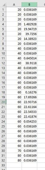
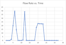
I have flow rate values in Column B that over a period of time has two spikes (B4:B7), and (B11:B12), before steadily rising for a period of time, before falling back down again. These relate to the various stages shown in Column A (stage 20,40,60,70 & 80).

Let's say in cell D2 I want code/formula to interrogate Column A & B, and based on Column A having not reached stage 60, look at Column B, recognise when the first spike starts (B4 - ie goes above 0.05), recognises when the spike is over (B7 as subsequent cell is back below 0.05), and then sums each cell in that range (B4,B5,B6 & B7), and returns the answer in D2.

I then want it to continue analysing Column B based on Column A not yet having reached 60, and do the same for the 2nd spike and return the sum in cell D3. I am not interested in anything after Column A reaches 60.

Had a bit of a mess about with some SUMIFS but couldn't get anything to work, and not even sure if that's the best way to go about it.

Can anyone help. Thanks

 

[dalvin647]

Hi David,

I don't think this is exactly what you're looking for, but it could be a stop-gap. I assumed that a spike cannot be through multiple stages, so I just did a sumifs based on >0.05 and the stage # - e.g. 20,40,60,70,80.

First Formula as so: =SUMIFS($B$1:$B$32,$A$1:$A$32,20,$B$1:$B$32,">0.05")

Book2
	A	B	C	D	E	F
1	20	0.036169		75.54495	20	<-Spikes
2	20	0.036169		39.55681	40
3	20	0.036169		108.4225	60
4	20	1.482928		0	70
5	20	19.94719		0	80
6	20	39.7256
7	20	14.38923
8	20	0.036169
9	40	0.036169
10	40	0.036169
11	40	0.645014
12	40	38.9118
13	40	0.036169
14	40	0.036169
15	40	0.036169
16	60	0.036169
17	60	0.036169
18	60	0.16276
19	60	17.69266
20	60	22.93716
21	60	22.61164
22	60	22.54533
23	60	22.41874
24	60	0.054253
25	60	0.036169
26	60	0.036169
27	60	0.036169
28	60	0.036169
29	60	0.036169
30	70	0.036169
31	80	0.036169
32	80	0.036169
Sheet1

Cell Formulas
Range	Formula
D1	D1	=SUMIFS($B$1:$B$32,$A$1:$A$32,20,$B$1:$B$32,">0.05")
D2	D2	=SUMIFS($B$1:$B$32,$A$1:$A$32,40,$B$1:$B$32,">0.05")
D3	D3	=SUMIFS($B$1:$B$32,$A$1:$A$32,60,$B$1:$B$32,">0.05")
D4	D4	=SUMIFS($B$1:$B$32,$A$1:$A$32,70,$B$1:$B$32,">0.05")
D5	D5	=SUMIFS($B$1:$B$32,$A$1:$A$32,80,$B$1:$B$32,">0.05")

 

[KRice]

Here is another idea that relies on some helper columns to 1) determine if the Stage and Flow Rate Threshold criteria are met (column D) and to 2) split the Flow Rate vs. Time curve into distinct Zones representing regions where the curve is below the threshold and above the threshold (column E). Then the summary block (in shaded green) uses formulas to determine the sum of each spike. I do not know whether it is possible for a spike to stretch across a "Stage". If so, the approach offered by @dalvin647 will capture partial sums of the spike within each of those Stages...but this might not be a realistic concern (you'll need to assess that). In this example, the two spikes occur in Zones 2 and 4.

MrExcel_20230523.xlsx
	A	B	C	D	E	F	G	H
1			Threshold >	0.05
2			Stage <	60
3
4	Time	Stage	Flow Rate	Criteria Met?	Zone		Zone	Sum
5	1	20	0.036169	FALSE	1		2	75.54495
6	2	20	0.036169	FALSE	1		4	39.55681
7	3	20	0.036169	FALSE	1
8	4	20	1.482928	TRUE	2
9	5	20	19.94719	TRUE	2
10	6	20	39.7256	TRUE	2
11	7	20	14.38923	TRUE	2
12	8	20	0.036169	FALSE	3
13	9	40	0.036169	FALSE	3
14	10	40	0.036169	FALSE	3
15	11	40	0.645014	TRUE	4
16	12	40	38.9118	TRUE	4
17	13	40	0.036169	FALSE	5
18	14	40	0.036169	FALSE	5
19	15	40	0.036169	FALSE	5
20	16	60	0.036169	FALSE	5
21	17	60	0.036169	FALSE	5
22	18	60	0.16276	FALSE	5
23	19	60	17.69266	FALSE	5
24	20	60	22.93716	FALSE	5
25	21	60	22.61164	FALSE	5
26	22	60	22.54533	FALSE	5
27	23	60	22.41874	FALSE	5
28	24	60	0.054253	FALSE	5
29	25	60	0.036169	FALSE	5
30	26	60	0.036169	FALSE	5
31	27	60	0.036169	FALSE	5
32	28	60	0.036169	FALSE	5
33	29	60	0.036169	FALSE	5
34	30	70	0.036169	FALSE	5
35	31	80	0.036169	FALSE	5
36	32	80	0.036169	FALSE	5
DavidWT87

Cell Formulas
Range	Formula
D5:D36	D5	=AND(B5<$D$2,C5>D$1)
E5:E36	E5	=IF(D5=D4,MAX(E$4:E4),MAX(E$4:E4)+1)
G5:G10	G5	=IFERROR(INDEX($E$5:$E$36,MATCH(1,(($D$5:$D$36)*($E$5:$E$36)>N(G4))*(COUNTIF(G$4:G4,$E$5:$E$36)=0),0)),"")
H5:H10	H5	=IFERROR(IF(AND(INDEX($D$5:$D$36,MATCH(G5,$E$5:$E$36,0)),G5<>""),SUMIF($E$5:$E$36,G5,$C$5:$C$36),""),"")
A5:A36	A5	=ROWS(A$5:A5)

 

[DavidWT87]

Here is another idea that relies on some helper columns to 1) determine if the Stage and Flow Rate Threshold criteria are met (column D) and to 2) split the Flow Rate vs. Time curve into distinct Zones representing regions where the curve is below the threshold and above the threshold (column E). Then the summary block (in shaded green) uses formulas to determine the sum of each spike. I do not know whether it is possible for a spike to stretch across a "Stage". If so, the approach offered by @dalvin647 will capture partial sums of the spike within each of those Stages...but this might not be a realistic concern (you'll need to assess that). In this example, the two spikes occur in Zones 2 and 4.

MrExcel_20230523.xlsx
	A	B	C	D	E	F	G	H
1			Threshold >	0.05
2			Stage <	60
3
4	Time	Stage	Flow Rate	Criteria Met?	Zone		Zone	Sum
5	1	20	0.036169	FALSE	1		2	75.54495
6	2	20	0.036169	FALSE	1		4	39.55681
7	3	20	0.036169	FALSE	1
8	4	20	1.482928	TRUE	2
9	5	20	19.94719	TRUE	2
10	6	20	39.7256	TRUE	2
11	7	20	14.38923	TRUE	2
12	8	20	0.036169	FALSE	3
13	9	40	0.036169	FALSE	3
14	10	40	0.036169	FALSE	3
15	11	40	0.645014	TRUE	4
16	12	40	38.9118	TRUE	4
17	13	40	0.036169	FALSE	5
18	14	40	0.036169	FALSE	5
19	15	40	0.036169	FALSE	5
20	16	60	0.036169	FALSE	5
21	17	60	0.036169	FALSE	5
22	18	60	0.16276	FALSE	5
23	19	60	17.69266	FALSE	5
24	20	60	22.93716	FALSE	5
25	21	60	22.61164	FALSE	5
26	22	60	22.54533	FALSE	5
27	23	60	22.41874	FALSE	5
28	24	60	0.054253	FALSE	5
29	25	60	0.036169	FALSE	5
30	26	60	0.036169	FALSE	5
31	27	60	0.036169	FALSE	5
32	28	60	0.036169	FALSE	5
33	29	60	0.036169	FALSE	5
34	30	70	0.036169	FALSE	5
35	31	80	0.036169	FALSE	5
36	32	80	0.036169	FALSE	5
DavidWT87

Cell Formulas
Range	Formula
D5:D36	D5	=AND(B5<$D$2,C5>D$1)
E5:E36	E5	=IF(D5=D4,MAX(E$4:E4),MAX(E$4:E4)+1)
G5:G10	G5	=IFERROR(INDEX($E$5:$E$36,MATCH(1,(($D$5:$D$36)*($E$5:$E$36)>N(G4))*(COUNTIF(G$4:G4,$E$5:$E$36)=0),0)),"")
H5:H10	H5	=IFERROR(IF(AND(INDEX($D$5:$D$36,MATCH(G5,$E$5:$E$36,0)),G5<>""),SUMIF($E$5:$E$36,G5,$C$5:$C$36),""),"")
A5:A36	A5	=ROWS(A$5:A5)

 

[DavidWT87]

Hello. Thanks, this looks like it's going to do exactly what I want it to do.

The only issue I'm having is the nothing is being returned in the zone/sum cells (the iferror formulas).

Is there anything you can see as to why it's not coming up? (The data is expanded more over what I posted initially - I took out a few rows here and there to make it a manageable set of data to talk around.

(I've also added in a couple of formula for my mass flow threshold, and bringing in the stage/flow rate data from another tab so that hopefully I can superimpose this calculation sheet into many different sets of data)

Copy of Test 36A 30.03.23 PASS.xlsm
	A	B	C	D	E	F	G	H
1		Mass Flow Rate Threshold >		0.03626898
2		Stage <		60
3
4	Time	Dispense Sequence Step	Mass_Flow Rate G/Sec	Criteria Met	Zone		Zone	Sum
5	1	0	0	FALSE	1
6	2	0	0	FALSE	1
7	3	0	0	FALSE	1
8	4	0	0	FALSE	1
9	5	0	0	FALSE	1
10	6	0	0	FALSE	1
11	7	0	0	FALSE	1
12	8	0	0	FALSE	1
13	9	0	0	FALSE	1
14	10	0	0	FALSE	1
15	11	0	0	FALSE	1
16	12	0	0	FALSE	1
17	13	0	0	FALSE	1
18	14	0	0	FALSE	1
19	15	0	0	FALSE	1
20	16	0	0	FALSE	1
21	17	20	0.03616898	FALSE	1
22	18	20	0.03616898	FALSE	1
23	19	20	0.03616898	FALSE	1
24	20	20	0.03616898	FALSE	1
25	21	20	1.482928	TRUE	2
26	22	20	19.94719	TRUE	2
27	23	20	39.7256	TRUE	2
28	24	20	14.38923	TRUE	2
29	25	20	0.03616898	FALSE	3
30	26	20	0.03616898	FALSE	3
31	27	20	0.03616898	FALSE	3
32	28	20	0.03616898	FALSE	3
33	29	20	0.03616898	FALSE	3
34	30	20	0.03616898	FALSE	3
35	31	20	0.03616898	FALSE	3
36	32	20	0.03616898	FALSE	3
37	33	20	0.03616898	FALSE	3
38	34	20	0.03616898	FALSE	3
39	35	20	0.03616898	FALSE	3
40	36	20	0.03616898	FALSE	3
41	37	20	0.03616898	FALSE	3
42	38	40	0.03616898	FALSE	3
43	39	40	0.03616898	FALSE	3
44	40	40	0.03616898	FALSE	3
45	41	40	0.6450135	TRUE	4
46	42	40	38.9118	TRUE	4
47	43	40	0.03616898	FALSE	5
48	44	40	0.03616898	FALSE	5
49	45	40	0.03616898	FALSE	5
50	46	40	0.03616898	FALSE	5
51	47	40	0.03616898	FALSE	5
52	48	40	0.03616898	FALSE	5
53	49	40	0.03616898	FALSE	5
54	50	40	0.03616898	FALSE	5
55	51	40	0.03616898	FALSE	5
56	52	60	0.03616898	FALSE	5
57	53	60	0.03616898	FALSE	5
Sheet4

Cell Formulas
Range	Formula
D1	D1	=C21+0.0001
B4:B57	B4	='RAW DATA'!AX1
C4:C57	C4	='RAW DATA'!BB1
A5:A57	A5	=ROWS(A$5:A5)
D5:D57	D5	=AND(B5<$D$2,C5>D$1)
E5:E57	E5	=IF(D5=D4,MAX(E$4:E4),MAX(E$4:E4)+1)
G5:G9	G5	=IFERROR(INDEX($E$5:$E$57,MATCH(1,(($D$5:$D$57)*($E$5:$E$57)>N(G4))*(COUNTIF(G$4:G4,$E$5:$E$57)=0),0)),"")
H5:H9	H5	=IFERROR(IF(AND(INDEX($D$5:$D$57,MATCH(G5,$E$5:$E$57,0)),G5<>""),SUMIF($E$5:$E$57,G5,$C$5:$C$57),""),"")

 

[KRice]

I have an idea...since you are using Excel 2016, array formulas are not natively handled unless you specify the formulas as such. Excel 365, which I am using, automatically recognizes the array formulas so the following steps are not necessary for the initial setup. I believe you may need to do this: Select cell G5, go to the formula bar at top and click F2 to enter into edit mode, then hit Ctrl-Shift-Enter to re-confirm the formula as an array formula. You should see curly brackets surround the formula in the formula bar. Then drag that formula down some appropriate number of cells (G5:G9 maybe?)...by clicking, holding, and dragging the small green rectangle that appears in the lower right corner of the cell when you select it. That should populate the G cells with the Zone numbers associated with the spikes. Do the same for the H column formula. And please let me know if that resolves the issue.

 

[DavidWT87]

I have an idea...since you are using Excel 2016, array formulas are not natively handled unless you specify the formulas as such. Excel 365, which I am using, automatically recognizes the array formulas so the following steps are not necessary for the initial setup. I believe you may need to do this: Select cell G5, go to the formula bar at top and click F2 to enter into edit mode, then hit Ctrl-Shift-Enter to re-confirm the formula as an array formula. You should see curly brackets surround the formula in the formula bar. Then drag that formula down some appropriate number of cells (G5:G9 maybe?)...by clicking, holding, and dragging the small green rectangle that appears in the lower right corner of the cell when you select it. That should populate the G cells with the Zone numbers associated with the spikes. Do the same for the H column formula. And please let me know if that resolves the issue.

Yes! That's done the job. Nice one

 

[KRice]

That’s great…I’m glad it’s working.