I have assumed that the range $H$17:$H$21 in your final formula in post 1 is an error as that range is 5 cells whereas the first two ranges are only 4 cells.
If that is correct and that should have been H17:H20 then try this in C1 copied across to D1, E1
Excel Formula:
=MATCH($A1,OFFSET($H1,COLUMNS($C1:C1)*8-8,0,4),0)
If you wanted to avoid the volatile function OFFSET then you could use this non-volatile alternative.
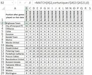
Sorry example was poor and badly explained. So new approach. Picture of data.
=MATCH($A2,sortuniques!$A$3:$A$21,0)
=MATCH($B2,sortuniques!$A$26:$A$44,0)
=MATCH($C2,sortuniques!$A$49:$A$67,0)
so D2 should be
=MATCH($D2,sortuniques!$A$72:$A$90,0)
ranges steps are constant 23 and 18. I have hard coded B2.C2.D2
I have dragged b2 down to B20 etc.
Need to drag b2 across the columns.
Hope that explains it better.
It is not clear whether they are formulas you have that are not working or formulas you want. Further, there is no indication of what cells they are or would be in.
Can you carefully insert the exact formulas you want in cells B2:D4 (9 cells) in your sheet, check that they are returning the results you expect, and then post those 9 formulas here, indicating which cell each formula is in.
My error again.
=MATCH($A2,sortuniques!$A$3:$A$21,0)
=MATCH($A2,sortuniques!$A$26:$A$44,0)
=MATCH($A2,sortuniques!$A$49:$A$67,0)
so D2 should be
=MATCH($A2,sortuniques!$A$72:$A$90,0)
My error again.
=MATCH($A2,sortuniques!$A$3:$A$21,0)
=MATCH($A2,sortuniques!$A$26:$A$44,0)
=MATCH($A2,sortuniques!$A$49:$A$67,0)
so D2 should be
=MATCH($A2,sortuniques!$A$72:$A$90,0)
I suspect that you may well be right, but that doesn't get the D2 formula to be matching in rows 72:90 as indicated by the OP in posts 5 and 7. I am guessing that the OP is just not being careful enough with precise information which is why I was trying to press that point.
We have a great community of people providing Excel help here, but the hosting costs are enormous. You can help keep this site running by allowing ads on MrExcel.com.
Allow Ads at MrExcel
Which adblocker are you using?
Disable AdBlock
Follow these easy steps to disable AdBlock
1)Click on the icon in the browser’s toolbar. 2)Click on the icon in the browser’s toolbar. 2)Click on the "Pause on this site" option.
Go back
Disable AdBlock Plus
Follow these easy steps to disable AdBlock Plus
1)Click on the icon in the browser’s toolbar. 2)Click on the toggle to disable it for "mrexcel.com".
Go back
Disable uBlock Origin
Follow these easy steps to disable uBlock Origin
1)Click on the icon in the browser’s toolbar. 2)Click on the "Power" button. 3)Click on the "Refresh" button.
Go back
Disable uBlock
Follow these easy steps to disable uBlock
1)Click on the icon in the browser’s toolbar. 2)Click on the "Power" button. 3)Click on the "Refresh" button.


")