Reformatting Margin Data with calculations

[snuffnchess]

I have put together a very small sampling of test data to show what I am trying to accomplish, but am not 100% of how to go about putting this in action.

We have a list of owners that pay a certain percent of margin of sales as a royalty payment. Which if it were just left at that it would be simple. There are then some exceptions where the percentages change based on the customer they are for etc. Then there are certain owners that we look back at a 3 week history for, and adjust numbers if the numbers have changed.

From the Fixed Data tab of the workbook, it will have the percentages, the exception accounts, minimum fees (if for some reason the minimum is not hit), and then column F to reflect if we are looking at the data from 3 weeks ago.

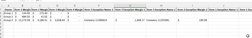
Current Tab has the margin in $ on it from current export and the margin for the exception accounts
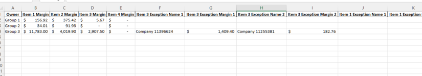
3 wk original tab has the margin in $ as it appeared 3 weeks ago on reports
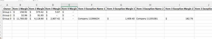
3 wk updated tab has the margin in $ as it appears today when looking at info from 3 weeks ago (there are sometimes adjustments that come in over time)

Desired result is ultimately how we want the data to look for the end result. (without the colors - i added those in just so that it was more obvious where the calculations came from).

Where do I even begin with this?


Fixed Data

Start.xlsx
	A	B	C	D	E	F	G	H	I	J	K	L	M	N	O	P	Q	R
1	Owner	Item 1	Item 3	Item 2	Item 4	3wk Comparison	Minimum	Min Waive	Alt Fee	Item 3 Exception % 1	Item 3 Exception % 2	Item 1 Exception Name 1	Item 1 Exception % 1	Item 1 Exception Name 2	Item 1 Exception % 2	Item 1 Exception Name 3	Item 1 Exception % 3	Notes
2	Group 1	18%	24%	15%	5%	n	$ 250.00
3	Group 2	18%	24%	15%	5%	y	$ 250.00
4	Group 3	17%	20%	17%	5%	y			$ 125.00	10%	10%
Fixed Data

Current

Start.xlsx
	A	B	C	D	E	F	G	H	I	J	K	L	M	N	O	P
1	Owner	Item 1 Margin	Item 2 Margin	Item 3 Margin	Item 4 Margin	Item 3 Exception Name 1	Item 3 Exception Margin 1	Item 3 Exception Name 2	Item 3 Exception Margin 2	Item 1 Exception Name 1	Item 1 Exception Margin 1	Item 1 Exception Name 2	Item 1 Exception Margin 2	Item 1 Exception Name 3	Item 1 Exception Margin 3	Notes
2	Group 1	$ 144.03	$ 175.40	$ -	$ -
3	Group 2	$ 684.55	$ 41.02	$ -	$ -
4	Group 3	$ 12,273.59	$ 4,186.31	$ 3,028.64	$ -	Company 11396624	$ 1,468.17	Company 11255381	$ 190.38
Current

3 wk Original

Start.xlsx
	A	B	C	D	E	F	G	H	I	J	K	L	M	N	O
1	Owner	Item 1 Margin	Item 2 Margin	Item 3 Margin	Item 4 Margin	Item 3 Exception Name 1	Item 3 Exception Margin 1	Item 3 Exception Name 2	Item 3 Exception Margin 2	Item 1 Exception Name 1	Item 1 Exception Margin 1	Item 1 Exception Name 2	Item 1 Exception Margin 2	Item 1 Exception Name 3	Item 1 Exception Margin 3
2	Group 1	$ 156.92	$ 375.42	$ 5.67	$ -
3	Group 2	$ 34.01	$ 91.93	$ -	$ -
4	Group 3	$ 11,783.00	$ 4,019.90	$ 2,907.50	$ -	Company 11396624	$ 1,409.40	Company 11255381	$ 182.76
3 Wk Original

3 wk Updated

Start.xlsx
	A	B	C	D	E	F	G	H	I	J	K	L	M	N	O
1	Owner	Item 1 Margin	Item 2 Margin	Item 3 Margin	Item 4 Margin	Item 3 Exception Name 1	Item 3 Exception Margin 1	Item 3 Exception Name 2	Item 3 Exception Margin 2	Item 1 Exception Name 1	Item 1 Exception Margin 1	Item 1 Exception Name 2	Item 1 Exception Margin 2	Item 1 Exception Name 3	Item 1 Exception Margin 3
2	Group 1	$ 156.92	$ 375.42	$ 5.67	$ -
3	Group 2	$ 32.96	$ 91.93	$ -	$ -
4	Group 3	$ 11,783.00	$ 4,118.90	$ 2,907.42	$ -	Company 11396624	$ 1,409.40	Company 11255381	$ 182.76
3 Wk Updated

Desired Result

Start.xlsx
	A	B	C	D	E	F	G	H	I	J	K
1
2		Owner	Description	Rate	Margin	Current Fee	Minimum	Adjustment	Alternate Fees	Invoice Total
3		Group 1				$ 319.43	$ 250.00			$ 319.43
4			Item 3	24%	$ -
5			Item 1	18%	$ 144.03
6			Item 2	15%	$ 175.40
7			Item 4	5%	$ -
8
9		Group 2
10			Item 3	15%	$ -	$ 725.57	$ 250.00	$ (1.05)		$ 724.52
11			Item 1	18%	$ 684.55
12			Item 2	15%	$ 41.02
13			Item 4	5%	$ -
14			Item 3 - Original	15%	$ -
15			Item 1 - Original	18%	$ 34.01
16			Item 2 - Original	15%	$ 91.93
17			Item 4 - Original	5%	$ -
18			Item 3 - Updated	15%	$ -
19			Item 1 - Updated	18%	$ 32.96
20			Item 2 - Updated	15%	$ 91.93
21			Item 4 - Updated	5%	$ -
22
23		Group 3
24			Item 3	20%	$ 3,028.64	$ 21,147.09		$ 98.92	$ 125.00	$ 21,371.01
25			Item 3 - Exc. 1	10%	$ 1,468.17
26			Item 3 - Exc. 2	10%	$ 190.38
27			Item 1	17%	$ 12,273.59
28			Item 2	17%	$ 4,186.31
29			Item 4	5%	$ -
30			Item 3 - Original	20%	$ 2,907.50
31			Item 3 - Exc. 1 - Original	10%	$ 1,409.40
32			Item 3 - Exc. 2 - Original	10%	$ 182.76
33			Item 1 - Original	17%	$ 11,783.00
34			Item 2 - Original	17%	$ 4,019.90
35			Item 4 - Original	5%	$ -
36			Item 3 - Updated	20%	$ 2,907.42
37			Item 3 - Exc. 1 - Updated	10%	$ 1,409.40
38			Item 3 - Exc. 2 - Updated	10%	$ 182.76
39			Item 1 - Updated	17%	$ 11,783.00
40			Item 2 - Updated	17%	$ 4,118.90
41			Item 4 - Updated	5%	$ -
42
Desired Result

Cell Formulas
Range	Formula
F3	F3	=SUM(E4:E7)
F10	F10	=SUM(E10:E13)
H10	H10	=SUM(E18:E21)-SUM(E14:E17)
J10	J10	=H10+F10
F24	F24	=SUM(E24:E29)
H24	H24	=SUM(E36:E41)-SUM(E30:E35)
J24	J24	=F24+H24+I24

 

[KRice]

Do you have any discretion to change the names of your column headings? I ask because a series of formulas could be used to extract information more easily if some relatively minor changes were made to facilitate matching desired content. Also, which version of Excel are you using? You can update your account details to show that. Certain functions available in Excel 365 would facilitate construction of your desired output, but if you're not using that version...

 

[snuffnchess]

Hi there. I will update my profile to reflect office 365. What type of changes do you think should be made to the headers? I do have discretion to change if needed. If the changes are major, I would just reformat the data that comes in to us via a macro so that it would match whatever is needed.

 

[snuffnchess]

Hello Kirk,

So sorry to be a pest - just wanted to see what it is that you had in mind for updating the data to make this work?

 

[KRice]

It's important provide sufficient clues so that each data element can be assigned to the correct category. In this case, a "category" means the intersection of a particular row and column in your Desired Result table. The Desired Result table has some columns that are to be taken directly from any of the other source tables (Owner, Description, Rate, Margin, Minimum, and Alternate Fees). Other columns in the Desired Result table are calculated from those just mentioned (Current Fee, Adjustment, and Invoice Total).

We also see in the Desired Result table that the rows involve groupings by Owner (Group 1, Group 2, etc.), then by Description. The Description labels appear to be sorted based on the sheet from which the data originate (with Fixed Data first followed by Current then by 3 Wk Original then by 2 Wk Updated). Within each subgrouping, further sorting appears to be based on the Fixed Data "rates" from largest to smallest (in this example, Item 3 at 0.24 followed by Items 1, 2, and 4.

To facilitate the categorization process, I looked for clues in the column headings, and most of them are okay. For example, margin "rates" are described in columns that include either the word "rate" or the "%" symbol, and those are used in the approach I'll describe below. The margin rates on the Fixed Data sheet do not include either of these clues, so I suggest adding "Rate" to them (I've done this in my sample file).

Rather than trying to pull data piecemeal from the various sheets, I think it makes sense to construct a large flat table that combines all of the information, assigns tags to it so that each element can be correctly mapped. Two ways to do this are with Power Query and VBA. I'm more comfortable with Power Query, but by most measures, I'm still a novice with it. In any case, I've taken a crack at transforming the tables and have gotten fairly close to your desired output, although there are a few things to consolidate and clean up...if I can figure it out, or perhaps someone will solve these trickier matters.

If you're not familiar with Power Query, it is a component of Excel that provides tools for operating on and transforming tables via a programming language (M-code). The first step is to transpose all of the source tables so that information pertaining to each owner appears in columns (rather than rows, as in the source tables).

A typical M-code script for this is:

let
    Source = Excel.CurrentWorkbook(){[Name="Table4"]}[Content],
    #"Demoted Headers" = Table.DemoteHeaders(Source),
    #"Transposed Table" = Table.Transpose(#"Demoted Headers"),
    #"Added Custom" = Table.AddColumn(#"Transposed Table", "Sheet", each "FixedData")
in
    #"Added Custom"

Here "Table4" is the default name Excel offered for the table on the FixedData sheet, and I simply accepted that name. This query is called FixedData, and three other very similar ones are Current, 3WkOrig, and 3WkUpdate, each transposing the tables on those similarly named sheets.

Then the main query called "Results" performs the task of appending the four transposed tables (stacking them on top of each other). An important assumption here is that the Owners are listed in the same order in all of the source tables, as the current code makes that assumption. Let me know if this assumption is problematic.

Then the long appended table is "unpivoted" so that all owner columns are stacked one over the other while keeping the values and attributes attached to them. Then a series of rules are applied to assign tags to each row to describe which column the value should appear in and where in the final output table should the row appear (this is where the word/symbol clues are critical). As mentioned previously, this query is a work in progress. The current output is show below (I left the helper columns in place that are used to sort by owner, tier (whether the data come from either of the 3Wk sheets), and within Tier2 (whether data come from 3WkOriginal or 3WkUpdated). In the final version, those columns will be removed before Power Query loads the table back onto the Results worksheet. I think they may be important to facilitate making the calculations in your Desired Results table.

The Results table has no formulas in it, as all of the operations to generate it are performed in the Power Query script. I still need to figure out how to move the value contents on the "Alt Fee" and "Minimum" rows to their corresponding "3wk Comparison" rows...and then the term "3Wk Comparison" will be changed to "Summary" or "Top Level" and will become the upper row for each Owner group.

With this approach, your tables are maintained normally, and when you want to generate a revised Results table, you would execute Data > Refresh All and the queries will execute and rebuild the Results table. For that reason, if formulas are used somewhere on the Results sheet, be sure:

1. The formulas can accommodate a potentially changing Results table structure (e.g., if some currently unused columns in the source tables are filled with data, new rows will appear in the Results table).
2. The formulas won't be overwritten when the new table is loaded.

You can get to the Query Editor via Data > Queries & Connections...and then hover the cursor over a query name and a popup window appears with Edit as an option...that is one way. Alternatively, click anywhere in the output table and then in the menu bar, click Query > Edit.

Sort.Owner	Sort.Tier	Sort.Tier2	Owner	Description	Rate	Margin	Minimum	Alternate Fees	Name	Comparison
1	1		Group 1	3wk Comparison						n
1	1		Group 1	Item 1	0.18	144.03				n
1	1		Group 1	Item 2	0.15	175.4				n
1	1		Group 1	Item 3	0.24	0				n
1	1		Group 1	Item 4	0.05	0				n
1	1		Group 1	Minimum			250			n
2	1		Group 2	3wk Comparison						y
2	1		Group 2	Item 1	0.18	684.55				y
2	1		Group 2	Item 2	0.15	41.02				y
2	1		Group 2	Item 3	0.24	0				y
2	1		Group 2	Item 4	0.05	0				y
2	1		Group 2	Minimum			250			y
2	2	1	Group 2	Item 1 - Original		34.01				y
2	2	1	Group 2	Item 2 - Original		91.93				y
2	2	1	Group 2	Item 3 - Original		0				y
2	2	1	Group 2	Item 4 - Original		0				y
2	2	2	Group 2	Item 1 - Updated		32.96				y
2	2	2	Group 2	Item 2 - Updated		91.93				y
2	2	2	Group 2	Item 3 - Updated		0				y
2	2	2	Group 2	Item 4 - Updated		0				y
3	1		Group 3	3wk Comparison						y
3	1		Group 3	Alt Fee				125		y
3	1		Group 3	Item 1	0.17	12273.59				y
3	1		Group 3	Item 2	0.17	4186.31				y
3	1		Group 3	Item 3	0.2	3028.64				y
3	1		Group 3	Item 3 - Exc. 1	0.1	1468.17			Company 11396624	y
3	1		Group 3	Item 3 - Exc. 2	0.1	190.38			Company 11255381	y
3	1		Group 3	Item 4	0.05	0				y
3	2	1	Group 3	Item 1 - Original		11783				y
3	2	1	Group 3	Item 2 - Original		4019.9				y
3	2	1	Group 3	Item 3 - Exc. 1 - Original		1409.4			Company 11396624	y
3	2	1	Group 3	Item 3 - Exc. 2 - Original		182.76			Company 11255381	y
3	2	1	Group 3	Item 3 - Original		2907.5				y
3	2	1	Group 3	Item 4 - Original		0				y
3	2	2	Group 3	Item 1 - Updated		11783				y
3	2	2	Group 3	Item 2 - Updated		4118.9				y
3	2	2	Group 3	Item 3 - Exc. 1 - Updated		1409.4			Company 11396624	y
3	2	2	Group 3	Item 3 - Exc. 2 - Updated		182.76			Company 11255381	y
3	2	2	Group 3	Item 3 - Updated		2907.42				y
3	2	2	Group 3	Item 4 - Updated		0				y

The current M-code that produced this table:

let
    Source = Table.Combine({FixedData, Current, #"3WkOrig", #"3WkUpdate"}),
    #"Trimmed Text" = Table.TransformColumns(Source,{{"Column1", Text.Trim, type text}}),
    #"Promoted Headers" = Table.PromoteHeaders(#"Trimmed Text", [PromoteAllScalars=true]),
    #"Changed Type" = Table.TransformColumnTypes(#"Promoted Headers",{{"Owner", type text}, {"Group 1", type any}, {"Group 2", type any}, {"Group 3", type any}, {"FixedData", type text}}),
    #"Filtered Rows" = Table.SelectRows(#"Changed Type", each ([Owner] <> "Owner")),
    #"Renamed Columns" = Table.RenameColumns(#"Filtered Rows",{{"FixedData", "Sheet"}}),
    #"Merged Columns" = Table.CombineColumns(#"Renamed Columns",{"Owner", "Sheet"},Combiner.CombineTextByDelimiter("/?/", QuoteStyle.None),"Merged"),
    #"Reordered Columns" = Table.ReorderColumns(#"Merged Columns",{"Merged", "Group 1", "Group 2", "Group 3"}),
    #"Unpivoted Columns" = Table.UnpivotOtherColumns(#"Reordered Columns", {"Merged"}, "Attribute", "Value"),
    #"Split Column by Delimiter" = Table.SplitColumn(#"Unpivoted Columns", "Merged", Splitter.SplitTextByDelimiter("/?/", QuoteStyle.Csv), {"Merged.1", "Merged.2"}),
    #"Changed Type1" = Table.TransformColumnTypes(#"Split Column by Delimiter",{{"Merged.1", type text}, {"Merged.2", type text}}),
    #"Renamed Columns1" = Table.RenameColumns(#"Changed Type1",{{"Merged.1", "CHeading"}, {"Merged.2", "Sheet"}, {"Attribute", "Owner"}}),
    #"Added Conditional Column" = Table.AddColumn(#"Renamed Columns1", "ValueTag", each if Text.Contains([CHeading], "Rate") then "Rate" else if Text.Contains([CHeading], "%") then "Rate" else if Text.Contains([CHeading], "Margin") then "Margin" else if Text.Contains([CHeading], "Minimum") then "Minimum" else if Text.Contains([CHeading], "Alt Fee") then "Alternate Fees" else if Text.Contains([CHeading], "Name") then "Name" else if Text.Contains([CHeading], "Comparison") then "Comparison" else null),
    #"Duplicated Column" = Table.DuplicateColumn(#"Added Conditional Column", "CHeading", "AttrTag"),
    #"Replaced Value1" = Table.ReplaceValue(#"Duplicated Column"," Rate","",Replacer.ReplaceText,{"AttrTag"}),
    #"Replaced Value2" = Table.ReplaceValue(#"Replaced Value1"," %","",Replacer.ReplaceText,{"AttrTag"}),
    #"Replaced Value3" = Table.ReplaceValue(#"Replaced Value2"," Margin","",Replacer.ReplaceText,{"AttrTag"}),
    #"Replaced Value4" = Table.ReplaceValue(#"Replaced Value3"," Name","",Replacer.ReplaceText,{"AttrTag"}),
    #"Replaced Value5" = Table.ReplaceValue(#"Replaced Value4","Exception","- Exc.",Replacer.ReplaceText,{"AttrTag"}),
    #"Added Conditional Column1" = Table.AddColumn(#"Replaced Value5", "AttrTag2", each if [Sheet] = "3WkUpdate" then [AttrTag]&" - Updated" else if [Sheet] = "3WkOrig" then [AttrTag]&" - Original" else [AttrTag]),
    #"Removed Columns" = Table.RemoveColumns(#"Added Conditional Column1",{"CHeading", "AttrTag"}),
    #"Added Conditional Column2" = Table.AddColumn(#"Removed Columns", "Sort.Tier", each if [Sheet] = "FixedData" then 1 else if [Sheet] = "Current" then 1 else 2),
    #"Grouped Rows" = Table.Group(#"Added Conditional Column2", {"Owner"}, {{"Grouping", each _, type table [Sheet=nullable text, Owner=text, Value=any, ValueTag=text, AttrTag2=text, Tier=number]}}),
    #"Added Index" = Table.AddIndexColumn(#"Grouped Rows", "Sort.Owner", 1, 1, Int64.Type),
    #"Expanded Grouping" = Table.ExpandTableColumn(#"Added Index", "Grouping", {"Sheet", "Value", "ValueTag", "AttrTag2", "Sort.Tier"}, {"Sheet", "Value", "ValueTag", "AttrTag", "Sort.Tier"}),
    #"Removed Columns1" = Table.RemoveColumns(#"Expanded Grouping",{"Sheet"}),
    #"Merged Columns1" = Table.CombineColumns(Table.TransformColumnTypes(#"Removed Columns1", {{"Sort.Owner", type text}, {"Sort.Tier", type text}}, "en-US"),{"Sort.Owner", "Sort.Tier", "Owner", "AttrTag"},Combiner.CombineTextByDelimiter("/?/", QuoteStyle.None),"Merged"),
    #"Pivoted Column" = Table.Pivot(#"Merged Columns1", List.Distinct(#"Merged Columns1"[ValueTag]), "ValueTag", "Value"),
    #"Split Column by Delimiter1" = Table.SplitColumn(#"Pivoted Column", "Merged", Splitter.SplitTextByDelimiter("/?/", QuoteStyle.Csv), {"Sort.Owner", "Sort.Tier", "Owner", "Description"}),
    #"Reordered Columns2" = Table.ReorderColumns(#"Split Column by Delimiter1",{"Sort.Owner", "Sort.Tier", "Owner", "Description", "Rate", "Margin", "Minimum", "Alternate Fees", "Name", "Comparison"}),
    #"Sorted Rows" = Table.Sort(#"Reordered Columns2",{{"Owner", Order.Ascending}, {"Description", Order.Ascending}}),
    #"Filled Down" = Table.FillDown(#"Sorted Rows",{"Comparison"}),
    #"Added Conditional Column3" = Table.AddColumn(#"Filled Down", "DeleteRow", each if Text.Contains([Description], "Original") and [Comparison] = "n" then 1 else if Text.Contains([Description], "Updated") and [Comparison] = "n" then 1 else null),
    #"Filtered Rows1" = Table.SelectRows(#"Added Conditional Column3", each ([DeleteRow] = null)),
    #"Removed Columns3" = Table.RemoveColumns(#"Filtered Rows1",{"DeleteRow"}),
    #"Added Conditional Column4" = Table.AddColumn(#"Removed Columns3", "Sort.Tier2", each if Text.Contains([Description], "Original") then 1 else if Text.Contains([Description], "Updated") then 2 else null),
    #"Reordered Columns1" = Table.ReorderColumns(#"Added Conditional Column4",{"Sort.Owner", "Sort.Tier", "Sort.Tier2", "Owner", "Description", "Rate", "Margin", "Minimum", "Alternate Fees", "Name", "Comparison"})
in
    #"Reordered Columns1"

No doubt, many improvements could be made to this script and approach. I hope to make further progress on it soon. Please let me know if you see any issues.

Because it is somewhat involved to get the scripts loaded and running, I've uploaded my file to Dropbox...available for download at:

Start.xlsx

Shared with Dropbox

www.dropbox.com

 

[snuffnchess]

Wow! Thank you for the thorough explanation. I am going to dig into your response tomorrow and get back to you.

Was hoping to do this in VBA, but open to learning power query as well, as there will be close to 200 owner accounts.

More to come tomorrow. Thank you again

 

[KRice]

With 200 owner accounts, you'll definitely want either Power Query or VBA. The latter might be the preferred approach, but I wouldn't be much help with it. I think with VBA the approach would be similar. Transpose all source tables (need to confirm that all owner accounts appear in the same order across the source tables?). Then append and tag...the Power Query script describes the approach I took to assign the tags. You could try out the current offering by cutting and pasting real info from your worksheets into the sample tables...and see if anything breaks.

 

[snuffnchess]

Hi Kirk... Seriously thank you for all of this work that you have put into this. I understand what you mean about the reformatting of the data, and this could definitely work. And I think I have found a way to incorporate CBA and power query together. I will say though that I am 100% unfamiliar with power query so it will be a process for sure.

I understand the logic behind it... just putting that logic into practice is where the issue comes in, if that makes sense.

 

[KRice]

I think the only changes I made to the source tables were the four headings shown here, where I added "Rate" so that the tag-assigning steps in the script could associate these columns with the Rate column in the Results table.

Owner	Item 1 Rate	Item 3 Rate	Item 2 Rate	Item 4 Rate

Are you able to confirm that the owners listed down column A on each sheet are in the same order on each sheet? If you follow the link I posted and download the Excel file, it includes the queries I described. You should be able to copy 10 or so rows of actual data from each of the four sheets in the official workbook and paste it directly into the corresponding tables in the sample file. Delete the three rows of sample data from each of the four tables, confirm that each of the tables have automatically resized to include your real data, and then execute Data > Refresh All, which should generate a new table on the Results sheet.

 

[snuffnchess]

The names would be the same on each sheet.... Is it easier / make more sense to do if the Margin amounts and the % are on the same worksheet? So for example if the data from the Fixed Data and Current worksheets were all in one row for each group?