Roster sum function question

[valtam]

Hello,

I am stumped on a roster I have been working on. There are several types of shifts for the workers, A, DD, S12 and so on. Each of those shifts has a numeric value, eg. DD = a 10 hour shift. So I'm guessing I need a table as a lookup reference like so?

Shift Code	Hours
A	8
DD	10
S12	12

<tbody>
</tbody>

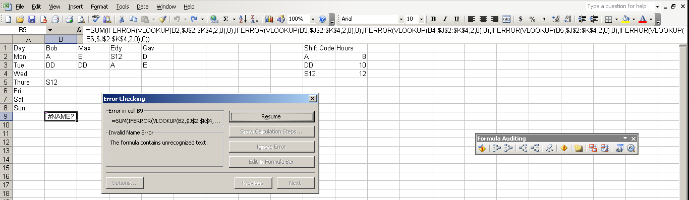
When I type in the Shift Codes in B2, B3 and B5 for example, I'd like B9 to show the total hours worked for Bob as a number. I'm having a hard time working out the formula that works best for this situation. Any guidance would be greatly appreciated. Thank you.

	A	B	C	D	E
1	Day	Bob	Max	Edy	Gav
2	Mon	A	E	S12	D
3	Tue	DD	DD	A	E
4	Wed
5	Thurs	S12
6	Fri
7	Sat
8	Sun
9		30	15	20	10

<tbody>
</tbody>

 

[FDibbins]

If you dont get a better answer (and Im positive you will, just cant think right now), give this brute-force option a try...
=SUM(IFERROR(VLOOKUP(B2,$J$2:$K$4,2,0),0),IFERROR(VLOOKUP(B3,$J$2:$K$4,2,0),0),IFERROR(VLOOKUP(B4,$J$2:$K$4,2,0),0),IFERROR(VLOOKUP(B5,$J$2:$K$4,2,0),0),IFERROR(VLOOKUP(B6,$J$2:$K$4,2,0),0))

I put your shiftcode/hours in J1:K4

 

[valtam]

Thanks for your help Ford, I used your formula and get the following error:

 

[Barbra]

Hey,

I tried to use FDibbins his code. And I noticed if you copy the code from his post there is a space (after the 2nd line; before the 3rd) where there shouldn't be one. I think that will solve your problem.

And I might have an other solution to your problem. Why don't you try:

=SUMPRODUCT((B2=$I$2:$I$6)*$J$2:$J$6)+SUMPRODUCT((B3=$I$2:$I$6)*$J$2:$J$6)+SUMPRODUCT((B4=$I$2:$I$6)*$J$2:$J$6)+SUMPRODUCT((B5=$I$2:$I$6)*$J$2:$J$6)+SUMPRODUCT((B6=$I$2:$I$6)*$J$2:$J$6)+SUMPRODUCT((B7=$I$2:$I$6)*$J$2:$J$6)+SUMPRODUCT((B8=$I$2:$I$6)*$J$2:$J$6)

Your Shiftcode/Hours are in I2:J6

Regards Barbra

PS: this was my first post and I hope this was helpfull.

 

[valtam]

Thank you Barbra, your solution worked - a great first post for you For the record, I did try the formula from Ford but without success, even with the correct copy format. Thank you to Ford as well for helping

 

[Barbra]

Glad I was able to help.

 

[daverm]

You can simplify Barbra's formula further to =SUMPRODUCT(((B2=$I$2:$I$6)+(B3=$I$2:$I$6)+(B4=$I$2:$I$6)+(B5=$I$2:$I$6)+(B6=$I$2:$I$6)+(B7=$I$2:$I$6)+(B8=$I $2:$I$6))*$J$2:$J$6)

I'm sure it can go neater than this though as well.

 

[valtam]

Thanks daverm, I like shorter code

 

[FDibbins]

Interesting that you say it did not work for you? (That extra space in IFERROR must have been a copy/paste error). I tried mu formula again and it works ok...

	A​	B​	C​	D​	E​	F​	G​	H​	I​	J​	K​
1​	Day​	Bob​	Max​	Edy​	Gav​					Shift Code​	Hours​
2​	Mon​	A​	E​	S12​	D​					A​	8​
3​	Tue​	DD​	DD​	A​	E​					DD​	10​
4​	Wed​	​	​	​	​					S12​	12​
5​	Thurs​	S12​	​	​	​
6​	Fri​	​	​	​	​
7​	Sat​	​	​	​	​
8​	Sun​	​	​	​	​
9​	Mine​	30​	10​	20​	0​
10​
11​	Yours​	30​	15​	20​	10​

B9=SUM(IFERROR(VLOOKUP(B2,$J$2:$K$4,2,0),0),IFERROR(VLOOKUP(B3,$J$2:$K$4,2,0),0),IFERROR(VLOOKUP(B4,$J$2:$K$4,2,0),0),IFERROR(VLOOKUP(B5,$J$2:$K$4,2,0),0),IFERROR(VLOOKUP(B6,$J$2:$K$4,2,0),0)) copied across

There is no matching code in column E, hence my total of 0