Shade cells based on content

[johnohio]

I am looking to create a spreadsheet that will color cells based on content.

Example...



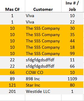
So basically it will shade the cell color based on the value in column A.. changing when the customer # changes.




Thanks for your help!

 

[Joe4]

Take a look at using Conditional Formatting, which allows you to format cells based on cell content. It can even reference other cells in the same row (i.e. you could Conditionally Format cell B1 based on the value in A1).

 

[Scott T]

This code will highlight every other customer number yellow.

Sub cf()
Dim lr As Long
lr = Cells(Rows.Count, 1).End(xlUp).Row
Range("A2:C" & lr).ClearFormats
For x = 3 To lr
    If Cells(x, 1) <> Cells(x - 1, 1) And Cells(x - 1, 1).Interior.Color <> vbYellow Then
        Range(Cells(x, 1), Cells(x, 3)).Interior.Color = vbYellow
    End If
    
    If Cells(x, 1) = Cells(x - 1, 1) And Cells(x - 1, 1).Interior.Color = vbYellow Then Range(Cells(x, 1), Cells(x, 3)).Interior.Color = Cells(x - 1, 1).Interior.Color
Next x

End Sub

 

[Joe4]

This code will highlight every other customer number yellow.

It looks like this assumes that the Customer numbers are in column A starting in row 2 and this column is sorted.

Under those same assumptions, you can do the same thing with Conditional Formatting, not requiring any VBA.
Just highlight rows 2 down to the end, and enter this Conditional Formatting formula:

=ISODD(SUMPRODUCT(1/COUNTIF($A$2:$A2,$A$2:$A2)))

and choose your formatting color.

 

[johnohio]

It looks like this assumes that the Customer numbers are in column A starting in row 2 and this column is sorted.

Under those same assumptions, you can do the same thing with Conditional Formatting, not requiring any VBA.
Just highlight rows 2 down to the end, and enter this Conditional Formatting formula:

=ISODD(SUMPRODUCT(1/COUNTIF($A$2:$A2,$A$2:$A2)))

and choose your formatting color.

Thanks that is perfect!

 

[Joe4]

You are welcome.