Shipping Calculator

[DataBlake]

Hello,
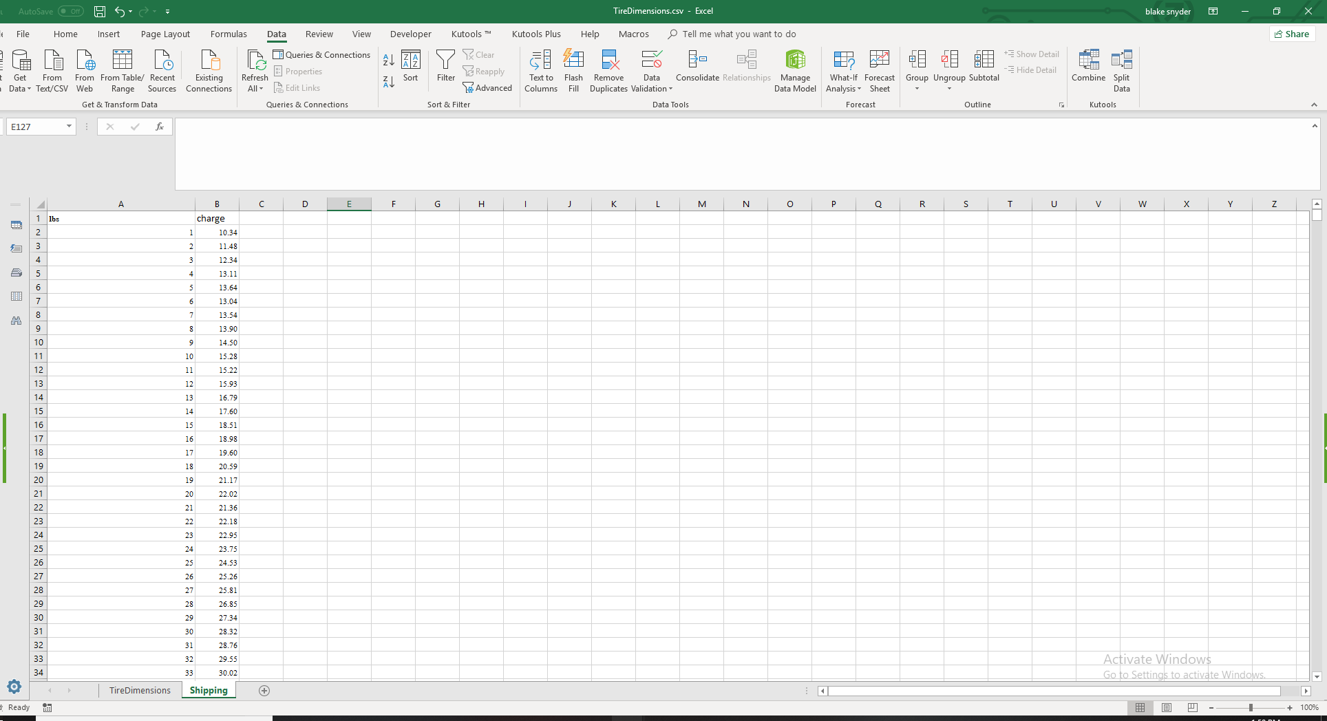
I have an issue where i have a shipping chart and want to use vlookup on the weight to grab a shipping price. the only thing is that anything past 150 lbs will be charged $0.47 per pound thats over 150. So lets say a have the weight in row B. B2 = 200. If B2 > 150 it needs to grab the value for the weight of 150 (lets say its sheet2!D153) and then add (50*0.47). 50 being the amount over 150 of the weight.

Any help would be greatly appreciated.

 

[mrshl9898]

We have a similar tool at work and use INDEX and MATCH to pull the rates through.

Here's an example, weight breaks up top (0-49,50-99,100-149 etc) and rates below

0	50	100	150	250	500	1000		160	0.5
0.6	0.5	0.4	0.3	0.25	0.2	0.15

<tbody>
</tbody>

Entering the weight I want a rate for in I1, the following formula returns the rate (0.5 in J1)

=INDEX(A1:G2,2,MATCH(I1,A1:G1))

In case you are unfamiliar "INDEX(A1:G2" defines the range I am looking in, the 2 means i'm looking in the 2nd row, and MATCH(I1,A1:G1) is finding the column for 160.

In the case of multiple rating locations you can substitute the 2 for a second match to return the row number containing the rate for a certain location.

 

[DataBlake]

okay yeah i understand this a little, i guess im just struggling with the references/lookup/arrays.
My sheets are column based instead of row based

So i want the weight (F2 even though i put G2) to match to the "lbs" column (shipping!A:A) and return the value of shipping!B:B
still confused as to how to make that formula you gave me reference that.

 

[DataBlake]

i feel like im close with
=INDEX(Shipping!$1:$1048576,0,2,MATCH(G2,Shipping!$1:$1048576))

=INDEX(Shipping!$A$2:$B$151,0,2,MATCH(G2,Shipping!$A$2:$A$151))
also doesn't work

 

[DataBlake]

i figured it out!
=INDEX(Shipping!$A$2:$B$151,MATCH(F2,Shipping!$A$2:$A$151),2)
i was under the impression that match was in the area and not the "column" so i just switched rows and columns

 

[DataBlake]

just in case this helps people this is my final formula:
=IF(F2>150,((F2-150)*0.47)+Shipping!$B$151,INDEX(Shipping!$A$2:$B$151,MATCH(F2,Shipping!$A$2:$A$151),2))