Paul_Nepomuceno
New Member
- Joined
- Oct 6, 2017
- Messages
- 6
[FONT="]Hi Guys,[/FONT]
[FONT="] [/FONT]
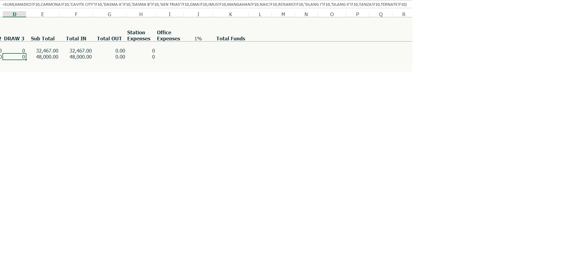
[FONT="]Is there anyway I can simplify this formula?[/FONT]
[FONT="] [/FONT]
[FONT="]B26 =SUM(AMADEO!F4,CARMONA!F4,'CAVITE CITY'!F4,'DASMA A'!F4,'DASMA B'!F4,'GEN TRIAS'!F4,GMA!F4,IMUS!F4,MANGAHAN!F4,NAIC!F4,ROSARIO!F4,'SILANG I'!F4,'SILANG II'!F4,TANZA!F4,TERNATE!F4)[/FONT]
[FONT="] [/FONT]
[FONT="]on B27 it should be like this =SUM(AMADEO!F8,CARMONA!F8,'CAVITE CITY'!F8,'DASMA A'!F8,'DASMA B'!F8,'GEN TRIAS'!F8,GMA!F8,IMUS!F8,MANGAHAN!F8,NAIC!F8,ROSARIO!F8,'SILANG I'!F8,'SILANG II'!F8,TANZA!F8,TERNATE!F8)[/FONT]
[FONT="]And so on. [/FONT]
[FONT="] [/FONT]
[FONT="]Is there a way to make this easier[/FONT]
[FONT="] [/FONT]
[FONT="]Thank you guys.[/FONT]
[FONT="] [/FONT]
[FONT="]Is there anyway I can simplify this formula?[/FONT]
[FONT="] [/FONT]
[FONT="]B26 =SUM(AMADEO!F4,CARMONA!F4,'CAVITE CITY'!F4,'DASMA A'!F4,'DASMA B'!F4,'GEN TRIAS'!F4,GMA!F4,IMUS!F4,MANGAHAN!F4,NAIC!F4,ROSARIO!F4,'SILANG I'!F4,'SILANG II'!F4,TANZA!F4,TERNATE!F4)[/FONT]
[FONT="] [/FONT]
[FONT="]on B27 it should be like this =SUM(AMADEO!F8,CARMONA!F8,'CAVITE CITY'!F8,'DASMA A'!F8,'DASMA B'!F8,'GEN TRIAS'!F8,GMA!F8,IMUS!F8,MANGAHAN!F8,NAIC!F8,ROSARIO!F8,'SILANG I'!F8,'SILANG II'!F8,TANZA!F8,TERNATE!F8)[/FONT]
[FONT="]And so on. [/FONT]
[FONT="] [/FONT]
[FONT="]Is there a way to make this easier[/FONT]
[FONT="] [/FONT]
[FONT="]Thank you guys.[/FONT]

")


