Stack multi columns in one column for visible cells only

[shafiey]

Why doesn't the formula work in column B when I change the range from A2:A1012 to A2:A2100?​

Formula in B2:
=IFERROR(SORT(FILTERXML("<t><s>" & SUBSTITUTE(TEXTJOIN("، ",,IF(SUBTOTAL(103,OFFSET(A2,ROW(A2:A1012)-ROW(A2),)),A2:A1012,"")),"، ","</s><s>") & "</s></t>","//s")),"")

Formula in C2:
=IFERROR(SORT(FILTERXML("<t><s>" & SUBSTITUTE(TEXTJOIN("، ",,IF(SUBTOTAL(103,OFFSET(A2,ROW(A2:A2100)-ROW(A2),)),A2:A2100,"")),"، ","</s><s>") & "</s></t>","//s")),"")

Why doesn't the formula work in column B when I change the range from A2:A1012 to A2:A2100?

My File

Thank you very much

 

[shafiey]

As far as I know: No


I did not edit any formula.

Can you explain, in words, what you are trying to do?

Thank you for taking the time for me.
I have two questions:
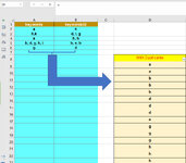
1- I have two text data columns with 3000 rows. Some data are multiple words in each cell and are separated by commas. I want all the data in the cells (A and B Columns) to be stack in one Column (for example D column) as a single word.
2- Also, after applying the filter on one of these two columns, the operation of step 1 should be performed on the visible cells, not on all the data.
I sent a sample file for better understanding. The problem with my main file is that it has many rows. Textjoin gives an error message: text too long.

I have MS Excel 2021.
Thank you

Example File


Before Filtering:

After Filtering:

 

[shafiey]

Thank you for taking the time for me.
I have two questions:
1- I have two text data columns with 3000 rows. Some data are multiple words in each cell and are separated by commas. I want all the data in the cells (A and B Columns) to be stack in one Column (for example D column) as a single word.
2- Also, after applying the filter on one of these two columns, the operation of step 1 should be performed on the visible cells, not on all the data.
I sent a sample file for better understanding. The problem with my main file is that it has many rows. Textjoin gives an error message: text too long.

I have MS Excel 2021.
Thank you

Example File


Before Filtering:
View attachment 98321

After Filtering:
View attachment 98322

will be corrected

‌Before Filtering:

 

[Peter_SSs]

I have two text data columns with 3000 rows. Some data are multiple words in each cell and are separated by commas.

As indicated before, this will likely cause TEXTJOIN to fail due to its character limit. I don't know of another option using standard worksheet functions that are available in your Excel version.
The result could certainly be achieved using vba. Would that be acceptable?

BTW, with your sample data, some items are separated by a comma and some are separated by a comma and a space. What is the circumstance with your actual data?

 

[shafiey]

You were exactly right. Also, it is possible to solve the problem with VBA, but I want to do it with a formula. My data is all comma separated. The problem can be solved with Office 360, but I have the 2021 version and I want to do it using the functions available in it. Finally, if I have to, I will use VBA with your help.
Thank you very much

 

[Peter_SSs]

What is the answer to my other question?

.. with your sample data, some items are separated by a comma and some are separated by a comma and a space. What is the circumstance with your actual data?

 

[Peter_SSs]

What is the answer to my other question?

Either way, you could give this a try.
I have assumed that the data is on Sheet1 and results go onto Sheet2 which exists but has nothing on it to start with.

On Sheet1 add the formula shown in C2 and copy down at least to the bottom of the data. Doesn't matter if the formula goes further as I have done.

shafiey.xlsm
	A	B	C
1	keywords	keywords02
2	a	h	2
3	h,k	d, i, g	2
4	a	h, h	2
5	b, d, g, h, i	b, e, b	2
6	g	d	2
7			0
8			0
Sheet1

Cell Formulas
Range	Formula
C2:C8	C2	=SUBTOTAL(103,A2:B2)

Now run the following macro. Post back if you need instructions about that.

Sub Make_List()
  Dim a As Variant, b As Variant, itm As Variant
  Dim i As Long
  
  With Sheets("Sheet1")
    a = .Range("A2:C" & .Columns("A:B").Find(What:="*", LookIn:=xlValues, SearchOrder:=xlByRows, SearchDirection:=xlPrevious).Row).Value
  End With
  With CreateObject("System.Collections.ArrayList")
    For i = 1 To UBound(a)
      If a(i, 3) > 0 Then
        For Each itm In Split(Replace(Application.TextJoin(",", 1, a(i, 1), a(i, 2)), " ", ""), ",")
          If Not .Contains(itm) Then .Add itm
        Next itm
      End If
    Next i
    .Sort
    If .Count > 0 Then b = Application.Transpose(.ToArray)
  End With
  With Sheets("Sheet2").Cells(1, Columns.Count).End(xlToLeft).Offset(, 1)
    .Value = .Offset(, -1).Value + 1
    If Not IsEmpty(b) Then .Offset(1).Resize(UBound(b) - LBound(b) + 1).Value = b
  End With
End Sub

Filter the data differently and run the macro again.
Each time the macro is run, the results are written to Sheet2 in a new column (the location can be changed to suit your requirements).
Here is my Sheet2 after I have run the macro 5 times. The top row just counts the number of times the macro has been run & could be removed from the code if not required.

1. First run was with nothing filtered out.
2. Second run I filtered out the "a" in column A
3. Third run I returned column A to Show All and filtered column B to show "d" only
4. Fourth run I returned both columns to Show All but then applied a text filter to show "x" in column B. This meant all rows except the heading row were hidden.
5. Fifth run I returned both columns to Show All

shafiey.xlsm
	A	B	C	D	E	F
1		1	2	3	4	5
2		a	b	d		a
3		b	d	g		b
4		d	e			d
5		e	g			e
6		g	h			g
7		h	i			h
8		i	k			i
9		k				k
10
Sheet2

 

[Anonymous1378]

You can try this wall of text:

Sheet1.xlsx
	A	B	C	D
1	keywords	keywords02
2	a	h
3	h,k	d, i, g
4	a	h, h
5	b, d, g, h, i	b, e, b
6	g	d
7
8				Result (no Blank & no Duplicate & Sort)
9				a
10				b
11				d
12				e
13				g
14				h
15				i
16				k
17
18
19
20
21
22
23
Sheet1

Cell Formulas
Range	Formula
D9:D16	D9	=LET( a,FILTER(A2:B6,SUBTOTAL(3,OFFSET(A2,ROW(A2:A6)-ROW(A2),0,1))), b,INDEX(a,MOD(SEQUENCE(COUNTA(a))-1,ROWS(a))+1,MOD(SEQUENCE(COUNTA(a))-1,2)+1), c,LEN(b)-LEN(SUBSTITUTE(b,",",""))+1, d,MMULT(--(SEQUENCE(ROWS(c))>=TRANSPOSE(SEQUENCE(ROWS(c)))),c), e,SEQUENCE(MAX(d)), f,XLOOKUP(e,d,d,,1), g,XMATCH(e,d,1), SORT(UNIQUE(FILTERXML("<t><s>" & SUBSTITUTE(INDEX(b,g),",","</s><s>") & "</s></t>","//s["&f-e+1&"]"))))
Dynamic array formulas.

 

[Peter_SSs]

You can try this wall of text:

Did you try it with data the size the OP has?

I have two text data columns with 3000 rows. Some data are multiple words in each cell and are separated by commas.

Admittedly, my machine is pretty old but with 2,000 rows of cells containing 3 words each (separated by comma only) I ran out of resources and could not complete.
Reducing the data to 2,000 rows with 2 words each, the task "completed" with no error message but more than 2,000 words were missing from the results.
In both cases my data was unfiltered.

 

[Anonymous1378]

Did you try it with data the size the OP has?



Admittedly, my machine is pretty old but with 2,000 rows of cells containing 3 words each (separated by comma only) I ran out of resources and could not complete.
Reducing the data to 2,000 rows with 2 words each, the task "completed" with no error message but more than 2,000 words were missing from the results.
In both cases my data was unfiltered.

I did not, prior to your comment, but I just tested it with 2,000 rows of 2 columns, 5 words each separated by comma only.

I did not run out of resources (32 GB RAM), but I noticed about 500 out of 4,300 words missing.

With a filter applied, surprisingly, it seemed to pick up about 4,250 words, except the ones I excluded.

Either way, probably not the most reliable approach, and am not too sure where the point of failure is. Hopefully it's some flaw in my logic which could just be pointed out rather than an inherent limitation of one of the functions being used.

 

[shafiey]

You can try this wall of text:

Sheet1.xlsx
	A	B	C	D
1	keywords	keywords02
2	a	h
3	h,k	d, i, g
4	a	h, h
5	b, d, g, h, i	b, e, b
6	g	d
7
8				Result (no Blank & no Duplicate & Sort)
9				a
10				b
11				d
12				e
13				g
14				h
15				i
16				k
17
18
19
20
21
22
23
Sheet1

Cell Formulas
Range	Formula
D9:D16	D9	=LET( a,FILTER(A2:B6,SUBTOTAL(3,OFFSET(A2,ROW(A2:A6)-ROW(A2),0,1))), b,INDEX(a,MOD(SEQUENCE(COUNTA(a))-1,ROWS(a))+1,MOD(SEQUENCE(COUNTA(a))-1,2)+1), c,LEN(b)-LEN(SUBSTITUTE(b,",",""))+1, d,MMULT(--(SEQUENCE(ROWS(c))>=TRANSPOSE(SEQUENCE(ROWS(c)))),c), e,SEQUENCE(MAX(d)), f,XLOOKUP(e,d,d,,1), g,XMATCH(e,d,1), SORT(UNIQUE(FILTERXML("<t><s>" & SUBSTITUTE(INDEX(b,g),",","</s><s>") & "</s></t>","//s["&f-e+1&"]"))))
Dynamic array formulas.

wow, That's ok. very very great, your formula worked.
Thank you very much.
Thank you very much for taking the time for me.
Is it possible to include repetitions in the column? Same as the following image: