Hello all -
I have a question, please:
Col A has values.
Col B checks a condition and returns true or not ("Y").
If Col B returns TRUE, Col C stores Col A's value.
Col D repeats the stored value so that:
Col E can check Col D against a different condition, and returns TRUE or not.
This contuinues until:
Col E returns TRUE ("condition met"), or
Col B (checking original condition) returns TRUE ("Y").
If Col B finds a new value has satisified the original condition, it stores that new value in Col C (and thus in D as well).
My problem is what to do with situations where Col E does not return true ("condition met") before a new value is stored in Col C and Col D.
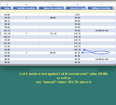
That "unused," value is still relevant, and may satisfy the condition in the future, so I need a way to keep track of these "unused," values and have Col E check both the current row against the running value in Col C (the regular operation), as well as against all other "unused," values from Col D above. In this example there is only one value (101.78) that has been "unused," but with more rows, there could be many "unused" values over time.
I have tried a number of ways to accomplish this, but none work. Is it possible to do this sort of thing, please? If so, any help will be very much appreciated, thank you!
I have a question, please:
Col A has values.
Col B checks a condition and returns true or not ("Y").
If Col B returns TRUE, Col C stores Col A's value.
Col D repeats the stored value so that:
Col E can check Col D against a different condition, and returns TRUE or not.
This contuinues until:
Col E returns TRUE ("condition met"), or
Col B (checking original condition) returns TRUE ("Y").
If Col B finds a new value has satisified the original condition, it stores that new value in Col C (and thus in D as well).
My problem is what to do with situations where Col E does not return true ("condition met") before a new value is stored in Col C and Col D.
That "unused," value is still relevant, and may satisfy the condition in the future, so I need a way to keep track of these "unused," values and have Col E check both the current row against the running value in Col C (the regular operation), as well as against all other "unused," values from Col D above. In this example there is only one value (101.78) that has been "unused," but with more rows, there could be many "unused" values over time.
I have tried a number of ways to accomplish this, but none work. Is it possible to do this sort of thing, please? If so, any help will be very much appreciated, thank you!
| The FO Q copy.xlsx | |||||||
|---|---|---|---|---|---|---|---|
| A | B | C | D | E | |||
| 1 | Value | Satisfies condition | Value that satisfied | Value Running | Different Condition | ||
| 2 | |||||||
| 3 | 82.00 | 0.00 | |||||
| 4 | 99.83 | Y | 99.83 | 99.83 | |||
| 5 | 99.12 | 99.83 | |||||
| 6 | 99.00 | 99.83 | |||||
| 7 | 99.60 | 99.83 | |||||
| 8 | 101.51 | 99.83 | condition met | ||||
| 9 | 101.78 | Y | 101.78 | 101.78 | |||
| 10 | 100.37 | 101.78 | |||||
| 11 | 99.68 | 101.78 | |||||
| 12 | 101.00 | 101.78 | |||||
| 13 | 91.00 | 101.78 | |||||
| 14 | 84.00 | 101.78 | |||||
| 15 | 85.00 | Y | 85.00 | 85.00 | |||
| 16 | 84.90 | 85.00 | |||||
| 17 | 86.00 | 85.00 | condition met | ||||
| 18 | 86.26 | 85.00 | |||||
Sheet1 | |||||||
| Cell Formulas | ||
|---|---|---|
| Range | Formula | |
| C3:C18 | C3 | =IF(B3="Y",A3,"") |
| D3:D18 | D3 | =IF(C3="",D2,C3) |
| E3:E18 | E3 | =IF(AND(A2<D3,A3>D3), "condition met","") |