Transpose & Blank Issues

[Data123]

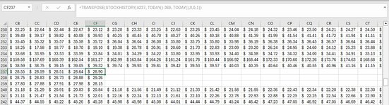
Hi when I use the =TRANSPOSE formula (see pic) I often get some blank rows. Those cells representing the blank rows have no formula. Meaning the formula is gone for those missing rows and this is what is causing it. I have created a new workbook and the same issue occurs again. I have verified those stocks have data.

Also, but less important why is the formula grayed out for the cell shown in the pic?

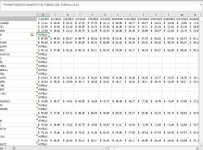
Oh one other question, for some reason when I get these blank areas and I try to refresh the data I the get many more blanks with the statement #SPILL! (see other pic).

 

[Peter_SSs]

Since my issue was that I had two formulas one that showed the date for price data and the other did not, does your second formula solve this issue and if so may I ask how?

Your original formula in cell B1 gave dates and prices for the stock SOXS on exchange ARCX. Since you have stock from other exchanges which may have different holidays/trading days the first formula may have excluded dates that are required to have full data for other exchanges/stocks.

The suggestions that I made produced dates independent of any exchange.
The first one in my previous post produces every date for a year so cannot "miss" any required dates.
The second suggestion in my previous post produces every date for a year except weekend dates. That also will not "miss" any required dates - unless one of the exchanges you are dealing with happens to trade on a weekend at some point. I don't know about that.
If you want all closing prices for a year then my first suggestion should give you that - and the second suggestion most likely will still give you that.

Since I need daily price data is it important that the dates be daily?

Unless I am misunderstanding the question, it really is a question for your, not me.

Why do you think TLST shows up in a worksheet, but not on the mini sheet upload?

Because there are limitations on how much mini sheet data can be included in a post I chose to only create the mini sheet as far as column AN for the first one and column AH for the second one.

Is it possible to verify what date a cells price data came from without a date header?

I think it is but would require vba. It also is not instant so there is a pause while the particular stock data is reloaded by the vba. Would those two restrictions be acceptable?
Also, why would you need this if you adopted one of my suggestions?

 

[Data123]

Your original formula in cell B1 gave dates and prices for the stock SOXS on exchange ARCX. Since you have stock from other exchanges which may have different holidays/trading days the first formula may have excluded dates that are required to have full data for other exchanges/stocks.

The suggestions that I made produced dates independent of any exchange.
The first one in my previous post produces every date for a year so cannot "miss" any required dates.
The second suggestion in my previous post produces every date for a year except weekend dates. That also will not "miss" any required dates - unless one of the exchanges you are dealing with happens to trade on a weekend at some point. I don't know about that.
If you want all closing prices for a year then my first suggestion should give you that - and the second suggestion most likely will still give you that.



Unless I am misunderstanding the question, it really is a question for your, not me.



Because there are limitations on how much mini sheet data can be included in a post I chose to only create the mini sheet as far as column AN for the first one and column AH for the second one.



I think it is but would require vba. It also is not instant so there is a pause while the particular stock data is reloaded by the vba. Would those two restrictions be acceptable?
Also, why would you need this if you adopted one of my suggestions?

Thanks Peter, you are awesome!!

 

[Peter_SSs]

You're welcome. Does that mean you are all set now?

 

[Data123]

You're welcome. Does that mean you are all set now?

I am on the data portion, but still working on the spreadsheet. I sure appreciate your help and others and I hope to see your input on my other questions. Excel is amazing, but I am new to it and like anything else it's a learning curve. So you don't use Excel for stocks research?

 

[Data123]

You're welcome. Does that mean you are all set now?

Hey Peter, I do have another question for you and I hope it's OK to ask you still. So I have a spreadsheet with three sheet tabs (+) at the bottom. Each sheet tab has the same symbol/name list (about 500+) as the spreadsheet. To make things easier to follow let's call the spreadsheet the dashboard. The dashboard simply has columns titled; name, symbol, price, volume and several price change %'s. So some of the dashboard's formulas connects to the other sheets data ie., price change %. So I noticed on the dashboard when I sort one of the "price change %" columns, I also choose to expand the sort to the other columns in the dashboard and the symbols shuffle as they should. However, the symbol list in the other sheets stay in their original order.

So my question for you is how can I put the dashboard symbol list back into it's original order to match the order of the symbol list of the other sheets (the original order is not alphabetical)? After reading this myself I realize how difficult it is to imagine. Please see below.

Please keep in mind the number of symbols I have (500+)

Spreadsheet/Dashboard after sorting and expanding a price change % column the other columns as well as the name/symbol list becomes mixed up.

Name
Ishares abcd
Quandrus mrfd
Charles tosd
Blackrock aksj

3 sheets (+) at the bottom of the Spreadsheet/dashboard has the original name/symbol list after I sorted the main spreadsheet/dashboard.

Name
Quandrus mrfd
Ishares abcd
Blackrock aksj
Charles tosd

*****Today I pressed ctrl-z many times to get the spreadsheet/dashboard symbol list back in order, but then had to redo many changes that were reversed. Thanks for your input!

 

[Peter_SSs]

I am on the data portion

OK, cheers.

Hey Peter, I do have another question ..

It is quite a different question so please start a new thread.

 

[Data123]

OK, cheers.


It is quite a different question so please start a new thread.

Will do.

 

[Data123]

You're welcome. Does that mean you are all set now?

Hi Peter, is there a way to show the most recent date first and the oldest date last when using the stockhistory function?

 

[Peter_SSs]

Sure, but it depends just what you are working with.

Example 1
A short stock history with dates ascending and below dates descending

Data123 Mr Excel Help_1.xlsm
	A	B	C	D	E	F	G	H	I	J	K
1	iShares:Tr Fl Rate Bond (ARCX:TFLO)	27/02/2024	28/02/2024	29/02/2024	1/03/2024	4/03/2024	5/03/2024	6/03/2024	7/03/2024	8/03/2024
2		$ 50.68	$ 50.68	$ 50.70	$ 50.50	$ 50.50	$ 50.52	$ 50.52	$ 50.55	$ 50.56
3
4	iShares:Tr Fl Rate Bond (ARCX:TFLO)	8/03/2024	7/03/2024	6/03/2024	5/03/2024	4/03/2024	1/03/2024	29/02/2024	28/02/2024	27/02/2024
5		$ 50.56	$ 50.55	$ 50.52	$ 50.52	$ 50.50	$ 50.50	$ 50.70	$ 50.68	$ 50.68
Sheet4

Cell Formulas
Range	Formula
B1:J2	B1	=TRANSPOSE(STOCKHISTORY(A1, TODAY()-14, TODAY(),0,0,0,1))
B4:J5	B4	=TRANSPOSE(SORT(STOCKHISTORY(A4, TODAY()-14, TODAY(),0,0,0,1),,-1))
Dynamic array formulas.

Example 2
However, if you were working with just dates at the top of the sheet as was the case at the beginning of this thread and suppose you were using my last example in post #9 where all dates for the year except weekends were used, then the stock history formula does not need to be altered at all, we only need to generate the date headings in descending order like this

Data123 Mr Excel Help_1.xlsm
	A	B	C	D	E	F	G	H	I	J	K	L	M	N	O	P	Q	R	S
1		12/03/2024	11/03/2024	8/03/2024	7/03/2024	6/03/2024	5/03/2024	4/03/2024	1/03/2024	29/02/2024	28/02/2024	27/02/2024	26/02/2024	23/02/2024	22/02/2024	21/02/2024	20/02/2024	19/02/2024	16/02/2024
2	iShares:MBS ETF (XNAS:MBB)			$ 92.93	$ 92.77	$ 92.60	$ 92.45	$ 91.78	$ 92.06	$ 91.91	$ 91.74	$ 91.47	$ 91.60	$ 91.80	$ 91.32	$ 91.26	$ 91.75		$ 91.68
3	LS ARKW TRACKER ETP (XLON:ARKB)			$ 259.03	$ 257.95	256.30	251.84	$ 258.73	$ 257.44	$ 254.52	$ 255.58	$ 250.28	245.49	240.29	$ 237.60	$ 234.71	$ 239.26	$ 248.74	$ 253.19
4	T-Rex 2X Long TESLA DT (XNAS:TSLT)			$ 11.34	$ 11.77	$ 11.52	$ 12.09	$ 13.15	$ 15.32	$ 15.20	$ 15.25	$ 14.91	$ 14.88	$ 13.81	$ 14.59	$ 14.25	$ 14.11		$ 15.06
Sheet5

Cell Formulas
Range	Formula
B1:JC1	B1	=LET(s,EDATE(TODAY(),-12)+1,d,SEQUENCE(,TODAY()-s+1,s),SORT(FILTER(d,WEEKDAY(d,2)<6),,-1,1))
B2:JC4	B2	=LET(sh,TRANSPOSE(STOCKHISTORY(A2, TODAY()-368, TODAY(),0,0,0,1)),IFNA(HLOOKUP(B$1#,sh,2,0),""))
Dynamic array formulas.

 

[Data123]

Sure, but it depends just what you are working with.

Example 1
A short stock history with dates ascending and below dates descending

*******Thanks Peter, that sort is extremely helpful!!!! Is there a version of this "=TRANSPOSE(SORT(STOCKHISTORY(A4, TODAY()-14, TODAY(),0,0,0,1),,-1))" without any header or "close", "date" statements? Meaning just the daily closing prices and nothing more? I have played with that formula for over an hour removing several of the parameters and even verified the ",0" for "no header" and it still shows a date header.