VBA or IF & OR function for algorithm

[jo_hivera]

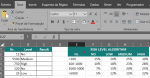
I need help automating an algorithm, where A is the Nr., that is freely inserted (i.e.: 12, 500, 175, 4, ...).
Cell C should recognize the number (as <100 to >5.000) from cell A, and the risk level accordingly on cell B, from No to High and present the result on cell C.
There is a second table with all the variables for this.

Is there a better/faster way, either VBA or i.e. IF function to do this?

 

[Fluff]

How about

+Fluff New.xlsm
	A	B	C	D	E	F	G	H	I
1	Nr	Level	Result
2	12	No	15%		Nr	No	Low	Medium	High
3	5500	Medium	15%		0	15%	20%	25%	30%
4	750	High	28%		101	10%	18%	23%	28%
5	120	No	10%		1001	7%	15%	20%	25%
6	25	Low	20%		5001	5%	12%	15%	22%
Rota

Cell Formulas
Range	Formula
C2:C6	C2	=INDEX($F$3:$I$6,MATCH(A2,$E$3:$E$6,1),MATCH(B2,$F$2:$I$2,0))

 

[jasonb75]

Just needs a basic index match function

Change the numbers in E3:E6 to 0, 100, 1000 and 5000, then enter the formula into C2 and fill down.

=IFERROR(INDEX($F$3:$I$6,MATCH($A2,$E$3:$E$6),MATCH($B2,$F$2:$I$2,0),"")

You may need to translate the function names to your own language and replace the commas with semicolons.

 

[jo_hivera]

Just needs a basic index match function

Change the numbers in E3:E6 to 0, 100, 1000 and 5000, then enter the formula into C2 and fill down.

=IFERROR(INDEX($F$3:$I$6,MATCH($A2,$E$3:$E$6),MATCH($B2,$F$2:$I$2,0),"")

You may need to translate the function names to your own language and replace the commas with semicolons.

Thank you so much! I gave it a try it only worked without the =IFERROR for some reason, seems to be working like a charm...

 

[jo_hivera]

How about

+Fluff New.xlsm
	A	B	C	D	E	F	G	H	I
1	Nr	Level	Result
2	12	No	15%		Nr	No	Low	Medium	High
3	5500	Medium	15%		0	15%	20%	25%	30%
4	750	High	28%		101	10%	18%	23%	28%
5	120	No	10%		1001	7%	15%	20%	25%
6	25	Low	20%		5001	5%	12%	15%	22%
Rota

Cell Formulas
Range	Formula
C2:C6	C2	=INDEX($F$3:$I$6,MATCH(A2,$E$3:$E$6,1),MATCH(B2,$F$2:$I$2,0))

Thank you so much! It worked like a charm!

 

[Fluff]

Glad we could help & thanks for the feedback.

 

[jasonb75]

it only worked without the =IFERROR for some reason,

Oops, typo caused that,

=IFERROR(INDEX($F$3:$I$6,MATCH($A2,$E$3:$E$6),MATCH($B2,$F$2:$I$2,0)),"")

 

[jo_hivera]

Oops, typo caused that,

=IFERROR(INDEX($F$3:$I$6,MATCH($A2,$E$3:$E$6),MATCH($B2,$F$2:$I$2,0)),"")

Ah! I was adding the ")" to try and fix it as well on the wrong side!
It's working! Thank you so much!