Vlookup, Index & Match - Grab values and compare

[cybid]

Greetings to all.
First of all, I am new to this forum and need the help of your excel knowledge.

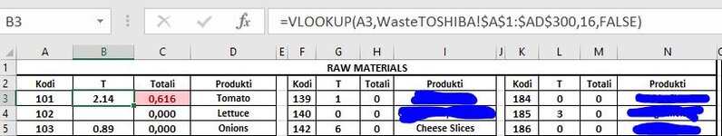
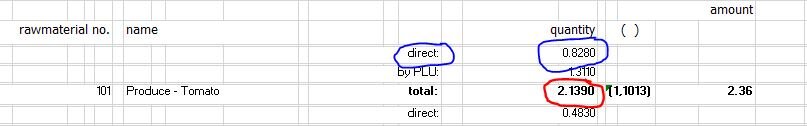
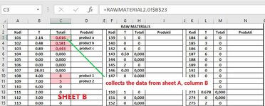
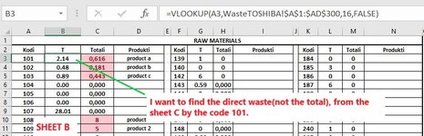
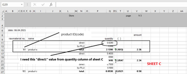
I have a workbook with the Sheets: A, B, C. On the B sheet I am collecting data from sheet A, and trying to collect other data from sheet C. Since the VLOOKUP wont collect negative col_index_num, I am trying to find a solution with index and match formula, but can't manage it. I am posting 2 images to give a visual of my problem. If you need other info or more details, please let me know and maybe I can upload the document for you. As you can see on the image number 2 I need to collect data with blue circle- only the value next to the 'direct:' text.

Thnx in advance.

 

[kvsrinivasamurthy]

Pl upload workbook (not doc) or clear images of sheets A , B and C. In sheet B where data is collected from Sheet A and C.

 

[cybid]

Pl upload workbook (not doc) or clear images of sheets A , B and C. In sheet B where data is collected from Sheet A and C.

I re-uploaded other screens hopping I did an understanding explanation.

 

[jasonb75]

Shouldn't need a workbook to answer this question.

Using the formula from your first screen capture as an example.

=VLOOKUP(A3,WasteTOSHIBA!$A$1:$AD$300,16,FALSE)

The INDEX and MATCH equivalent would be

=INDEX(WasteTOSHIBA!$P$1:$P$300,MATCH(A3,WasteTOSHIBA!$A$1:$A$300,FALSE))

The index range, P1:P300 is the result column (column 16) from the original formula. The match range is the left column. Regardless of the columns involved for the result to return and the criteria, the format of the formula is the same.

Remember that match must always be a single column (or row), index should also be a single column (or row) unless you are using 2 separate matches (1 for row, another for column), although I suggest that you familiarise yourself with the single match method first.

 

[cybid]

Shouldn't need a workbook to answer this question.

Using the formula from your first screen capture as an example.

=VLOOKUP(A3,WasteTOSHIBA!$A$1:$AD$300,16,FALSE)

The INDEX and MATCH equivalent would be

=INDEX(WasteTOSHIBA!$P$1:$P$300,MATCH(A3,WasteTOSHIBA!$A$1:$A$300,FALSE))

The index range, P1:P300 is the result column (column 16) from the original formula. The match range is the left column. Regardless of the columns involved for the result to return and the criteria, the format of the formula is the same.

Remember that match must always be a single column (or row), index should also be a single column (or row) unless you are using 2 separate matches (1 for row, another for column), although I suggest that you familiarise yourself with the single match method first.

Hey jasconb, thnnx for the help but still not getting the desired value from Sheet C.

I wanna be able to grab the cell P11 and not the P15 which matches the code 101.

As you can see on the image named DOC C.1, I have circled the cell which I'm trying to grab and put on docB.

 

[jasonb75]

Based on that,

=INDEX(WasteTOSHIBA!$P$1:$P$300,MATCH(A3,WasteTOSHIBA!$A$5:$A$304,FALSE))

This assumes that the value to 'grab' will always be 4 rows above the code to match, although looking at the was that the sheet is laid out, I would expect any formula to fail.

 

[cybid]

Based on that,

=INDEX(WasteTOSHIBA!$P$1:$P$300,MATCH(A3,WasteTOSHIBA!$A$5:$A$304,FALSE))

This assumes that the value to 'grab' will always be 4 rows above the code to match, although looking at the was that the sheet is laid out, I would expect any formula to fail.

jasonb75 I am thankful to your help. It's working great and will do a lot of work. Thank You

 

[cybid]

Based on that,

=INDEX(WasteTOSHIBA!$P$1:$P$300,MATCH(A3,WasteTOSHIBA!$A$5:$A$304,FALSE))

This assumes that the value to 'grab' will always be 4 rows above the code to match, although looking at the was that the sheet is laid out, I would expect any formula to fail.

Hey jason, I have another question for this formula. Is there an option to put an IF condition like: If there is direct: for product ID 101 grab that direct value, but if there isn't any direct value for product ID 101 put 0.
I hope I explained correct.
Thnx in advance.

 

[jasonb75]

You mean error trap it so that it doesn't show #N/A when the ID is not found?

=IFERROR(INDEX(WasteTOSHIBA!$P$1:$P$300,MATCH(A3,WasteTOSHIBA!$A$5:$A$304,FALSE)),0)

 

[cybid]

Where I work, we use a program which generates the usage of products daily. But sometimes a product does not have a direct value, so when using the formula it grabs the upper product's value. For example Product A has a direct: value 0.8280 as shown on the screenshot SHEET C. But if the Product B does not have the direct: value, the formula grabs the total value of product above. And the question is: If product B does not have a direct: value can the formula put 0 on sheet B?

Thanks again on your support.