vlookup, INDEX, or SUMPRODUCT???

revampeng

New Member
Joined
Mar 7, 2024
Messages
6
Office Version
  1. 365
Platform
  1. Windows
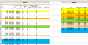
This hopefully comes through okay. I am looking to automate the information going into columns G and H. I highlighted the date ranges to make this a bit clearer. In the real world I will have "Source 2" with samples every 10 minutes. "Source 1" is just whenever a fault occurs. The goal is to move the temperature and humidity that matches the date and time (within the 10 minute sample window) into those column G and H cells. For example if we look at March 1, 2024 on Source 2 I would want the 74.31 to go to G8 and 43.4 to go to H8. I have been toying with vlookup and I am struggling since the data sets are different sizes and the times will not line up due to the 10 minute sampling.

Hopefully this makes sense; let me know if it doesn't.

Question Example.xlsx
ABCDEFGHIJKLMNO
1Source 1Source 2
2
3F770 :Barcode Printer Error(14ST) and F773 :Printer Cycle Time Over(14ST)
4F-CodeF-Code Counts
5dateTime770773770 Count773 CountTemp °FHumidity %No.TimeTemperature°FHumidity%
6Friday, March 1, 202410:25:47 AM7707730012024-03-01 17:20:0073.8146.0
7Friday, March 1, 202412:30:38 PM7707730022024-03-01 17:30:0073.9245.8
8Friday, March 1, 20245:49:49 PM7707731032024-03-01 17:40:0074.3143.4
9Friday, March 1, 20246:40:30 PM7707731042024-03-01 17:50:0074.1044.4
10Friday, March 1, 20248:45:18 PM770773002202024-03-02 23:10:0073.8046.0
11Friday, March 1, 20249:05:26 PM770773102212024-03-02 23:20:0073.9045.8
12Friday, March 1, 202410:22:50 PM770773002222024-03-02 23:30:0074.4043.5
13Saturday, March 2, 202411:13:19 PM770773102232024-03-02 23:40:0074.3044.4
14Saturday, March 2, 202411:21:17 PM770773107512024-03-04 05:20:0074.2543.1
15Saturday, March 2, 202411:47:34 PM770773107522024-03-04 05:30:0074.3642.4
16Saturday, March 2, 202411:51:58 PM770773107532024-03-04 05:40:0074.4741.7
17Saturday, March 2, 20241:10:38 AM770773107542024-03-04 05:50:0074.5840.9
18Monday, March 4, 20245:14:03 AM7707730012102024-03-05 06:10:0074.6940.2
19Monday, March 4, 20245:21:30 AM7707731012112024-03-05 06:20:0073.8339.5
20Monday, March 4, 20245:30:15 AM7707731012122024-03-05 06:30:0073.9538.8
21Monday, March 4, 20245:33:19 AM7707731012132024-03-05 06:40:0075.0238.1
22Monday, March 4, 20245:40:51 AM7707730013202024-03-06 07:10:0075.1337.3
23Monday, March 4, 20245:44:28 AM7707731013212024-03-06 07:20:0075.2436.6
24Monday, March 4, 20246:04:54 AM7707730013222024-03-06 07:30:0073.5035.9
25Monday, March 4, 20246:07:06 AM7707731013252024-03-06 07:40:0072.7035.2
26Tuesday, March 5, 20246:17:46 AM77077310
27Tuesday, March 5, 20246:29:23 AM77077310
28Tuesday, March 5, 20246:35:09 AM77077310
29Tuesday, March 5, 20247:19:49 AM77077310
30Wednesday, March 6, 20247:21:33 AM77077310
31Wednesday, March 6, 20247:23:19 AM77077310
32Wednesday, March 6, 20247:24:01 AM77077310
33Wednesday, March 6, 20247:25:16 AM77077300
34Thursday, March 7, 20247:28:54 AM77077310
35Thursday, March 7, 20247:43:11 AM77077310
36Friday, March 8, 20247:50:22 AM77077300
37Friday, March 8, 20248:04:17 AM77077310
38Friday, March 8, 20248:17:45 AM77077310
39Saturday, March 9, 20248:18:47 AM77077300
40Saturday, March 9, 20248:22:13 AM77077310
Sheet1
 

Attachments

  • Question Example.PNG
    Question Example.PNG
    96.4 KB · Views: 4

Excel Facts

Can a formula spear through sheets?
Use =SUM(January:December!E7) to sum E7 on all of the sheets from January through December
Welcome to the Forum!

Try G6:=LET(t,A6+B6,s,M$6:M$25,m,MATCH(t,s,1),IFERROR(IF(t-INDEX(s,m)<=1/144,INDEX(N$6:O$25,m,),""),""))

Consistent with your example, this takes the previous (rather than closest) Source 2 data, if it's within 10 minutes of the fault time.
 
Upvote 0
@StephenCrump that worked. Really appreciate your help. Now I need to digest this formula, I am admittedly lost as to why it works currently.
 
Upvote 0
Welcome to the Forum!

Try G6:=LET(t,A6+B6,s,M$6:M$25,m,MATCH(t,s,1),IFERROR(IF(t-INDEX(s,m)<=1/144,INDEX(N$6:O$25,m,),""),""))

Consistent with your example, this takes the previous (rather than closest) Source 2 data, if it's within 10 minutes of the fault time.
Where did it come from or what is the <=1/144? I have never used the LET function, that is sweet; thanks for this lesson.
 
Upvote 0
I don't see Stephen online at the moment, but in order to not keep you waiting any longer...the formula uses the LET function, which allows us to assign variable names to cell references, ranges, or even other functions. This is advantageous because it can reduce redundancy when the same quantity is used several times in subsequent calculations. It also allows us to construct intermediate results and assign them to variables that are used later, without needing to stash those values in helper cells somewhere.

A quick review: Excel treats dates as a number relative to some baseline "0" date (and that 0 date is system dependent, as MacOS and Windows versions of Excel use different 0 dates). Bottom line though is that a calendar day will have an integer value. Time is treated as some fractional part of a day, so 8:00 AM is 0.3333 and 12:00 PM (noon) is 0.5. The "t" variable is then the date/time combination--the sum of date and time--a single value that tells us both the date and the time in the Source 1 table, and this value directly corresponds to the list in the "Time" column of Source 2, which are actually date/time combinations too. The date/times in Source 2 are assigned to variable "s", an array of date/time values. Then a MATCH is performed to determine which row index in "s" (the Source 2 date/time values) occurred just before or at exactly the same time as the Source 1 "t" value. This is done with the MATCH function using the "1" option (the 3rd argument) to instruct the function to find the largest value in the lookup array that is smaller than or equal to the lookup value. MATCH returns the row index (the list position in the "s" array) where the match is found, and this row index is assigned to the "m" variable. Then the final check is made: there are six 10-minute blocks of time in an hour, and 24 hours in a day, so there are 6*24=144 10-minute blocks in a full day. So the Source 2 date/time is subtracted from the Source 1 date/time to determine the fractional part of a day that separates those two instances. I believe you want to ensure that the data pulled from Source 2 occurred within 10 minutes of the Source 1 date/time, so the IF statement checks whether the difference is less than or equal to 1/144 (the fractional part of a day corresponding to 10 minutes), and if that is true, the Temperature and Humidity from Source 2 is delivered by the INDEX function, otherwise a blank is returned.
 
Upvote 1
@StephenCrump or @KRice Is there a limit in range to the LET function. In the "real world" use of the below formula I will have a separate "dump sheet" where I will copy in the raw data from the data logger; hence the "Sheet2!" in the ranges now. "Source 2 -- Date & Time Separated" which is the same data as Sheet2!B6:E45 shown in the XL2BB Mini Sheet. What I ran into is that the formula works with the range B6:B45. But it returns a blank if I increase the range to B6:B46. I noticed this on the actual workbook where I made the range B6:B40000 and nothing happened. The XL2BB Mini Sheet below is the actual raw data from today; the B column is the same as column Q, C = R, D = S, and E = T should you need to change the formula.

Basically I am needing a limitless range for the formula. The sheet gets renewed every year, best guess is I will have 40,000 entries per year. Didn't know if this formula would work with B:B or if it needed any actual range. Or if I can use COUNTA somehow to find the bottom of the table? I will try that while I await a reply.

=LET(t,A7+B7,s,Sheet2!$B$6:$B$45+Sheet2!$C$6:$C$45,m,MATCH(t,s,1),IFERROR(IF(t-INDEX(s,m)<=1/144,INDEX(Sheet2!$D$6:Sheet2!$E$45,m,),""),""))

Question Example -- Real Raw Data.xlsx
ABCDEFGHIJKLMNOPQRST
1Source 1Source 2Source 2 -- Date & Time Separated
2
3F770 :Barcode Printer Error(14ST) and F773 :Printer Cycle Time Over(14ST)
4F-CodeF-Code Counts
5dateTime770773770 Count773 CountTemp °FHumidity %No.TimeTemperature°FHumidity%dateTimeTemperature°FHumidity%
62024-03-0813:08:5977077300 1802024-03-08 17:41:5178.444.22024-03-0817:41:5178.4044.20
72024-03-0817:47:377707730078.4044.201812024-03-08 17:51:5178.842.12024-03-0817:51:5178.8042.10
82024-03-0818:01:037707730078.8042.101822024-03-08 18:01:517941.92024-03-0818:01:5179.0041.90
92024-03-0818:12:117707730078.4044.401832024-03-08 18:11:5178.444.42024-03-0818:11:5178.4044.40
102024-03-0818:13:307707730078.4044.401842024-03-08 18:21:5179.241.52024-03-0818:21:5179.2041.50
112024-03-0818:14:077707730078.4044.401852024-03-08 18:31:5179.241.82024-03-0818:31:5179.2041.80
122024-03-0818:14:517707730078.4044.401862024-03-08 18:41:5179.341.82024-03-0818:41:5179.3041.80
132024-03-0818:15:287707731078.4044.401872024-03-08 18:51:5179.3NC2024-03-0818:51:5179.30NC
142024-03-0818:16:127707731078.4044.401882024-03-08 19:01:5179.3NC2024-03-0819:01:5179.30NC
152024-03-0818:52:077707730079.30NC1892024-03-08 19:11:5179.242.92024-03-0819:11:5179.2042.90
162024-03-0819:24:147707730079.3043.501902024-03-08 19:21:5179.343.52024-03-0819:21:5179.3043.50
172024-03-0819:51:507707730079.5042.201912024-03-08 19:31:5179.541.92024-03-0819:31:5179.5041.90
182024-03-0820:22:587707730079.3043.601922024-03-08 19:41:5179.542.22024-03-0819:41:5179.5042.20
192024-03-0820:23:137707730079.3043.601932024-03-08 19:51:5179.541.82024-03-0819:51:5179.5041.80
202024-03-0821:39:2677077300 1942024-03-08 20:01:5179.741.82024-03-0820:01:5179.7041.80
212024-03-0822:59:2477077300 1952024-03-08 20:11:5179.7412024-03-0820:11:5179.7041.00
222024-03-090:07:2077077300 1962024-03-08 20:21:5179.343.62024-03-0820:21:5179.3043.60
232024-03-091:55:3877077310 1972024-03-08 20:31:5179.741.92024-03-0820:31:5179.7041.90
242024-03-115:10:3477077300 1982024-03-08 20:41:5179.940.62024-03-0820:41:5179.9040.60
252024-03-117:17:0377077300 1992024-03-08 20:51:5179.940.92024-03-0820:51:5179.9040.90
Sheet1
Cell Formulas
RangeFormula
Q6:Q25Q6=INT(M6)
R6:R25R6=MOD(M6,1)
S6:T25S6=N6
G6,G8:H25G6=LET(t,A6+B6,s,Sheet2!$B$6:$B$25+Sheet2!$C$6:$C$25,m,MATCH(t,s,1),IFERROR(IF(t-INDEX(s,m)<=1/144,INDEX(Sheet2!$D$6:Sheet2!$E$25,m,),""),""))
G7:H7G7=LET(t,A7+B7,s,Sheet2!$B$6:$B$45+Sheet2!$C$6:$C$45,m,MATCH(t,s,1),IFERROR(IF(t-INDEX(s,m)<=1/144,INDEX(Sheet2!$D$6:Sheet2!$E$45,m,),""),""))
Dynamic array formulas.
 
Upvote 0
If I haven't messed it up too much, this variation of the formula might help:
Excel Formula:
=LET(t,A21+B21,ref,Sheet2!$B:$E,lrow,LOOKUP(2,1/(TAKE(ref,,1)<>""),ROW(TAKE(ref,,1))),data,TAKE(ref,lrow),s,CHOOSECOLS(data,1)+CHOOSECOLS(data,2),m,MATCH(t,s,1),
IFERROR(IF(t-INDEX(s,m)<=1/144,INDEX(TAKE(data,,-2),m,),""),""))
For convenience, the full column range reference for the reference data is assigned to the "ref" variable. Then we find the last occupied cell of the first column of "ref" (in this case, Sheet2's column B) and assign that value to the variable "lrow"...last row. Then we trim down the size of the lookup data with the "data" formula, so we TAKE(ref,lrow), and then refer to various columns in the "data" array for the rest of the formula. This should dynamically adapt in size for new data dumps.
 
Upvote 1
Solution
If I haven't messed it up too much, this variation of the formula might help:
Excel Formula:
=LET(t,A21+B21,ref,Sheet2!$B:$E,lrow,LOOKUP(2,1/(TAKE(ref,,1)<>""),ROW(TAKE(ref,,1))),data,TAKE(ref,lrow),s,CHOOSECOLS(data,1)+CHOOSECOLS(data,2),m,MATCH(t,s,1),
IFERROR(IF(t-INDEX(s,m)<=1/144,INDEX(TAKE(data,,-2),m,),""),""))
For convenience, the full column range reference for the reference data is assigned to the "ref" variable. Then we find the last occupied cell of the first column of "ref" (in this case, Sheet2's column B) and assign that value to the variable "lrow"...last row. Then we trim down the size of the lookup data with the "data" formula, so we TAKE(ref,lrow), and then refer to various columns in the "data" array for the rest of the formula. This should dynamically adapt in size for new data dumps.
Is this what you do for a living? I am just a dumb Production Engineer, and haven't been in Excel much in the last 12 years. Very basic vlookups and such is the extent of what I have needed.

Other than the 3 minutes to calculate the 40,000 cells, this did the trick. Much appreciated sir. Now to study the formula and understand all the ins and outs.
 
Upvote 0
No...retired engineer now. Glad to hear it's working, although I was worried that it might be sluggish. I normally try to avoid full column references because they can be slow. I'm not sure which steps are most responsible for the sluggishness, but you could experiment. For one, you could redefine "ref" with a smaller, but still overly large range...something like
Excel Formula:
Sheet2!$B1:$E60000
to immediately trim down the initial range that needs to be searched for the last non-empty cell. And you could use COUNTA, which might be faster than LOOKUP...although you need to be aware of how COUNTA is working. It counts nonblank cells in some column. So any blanks interspersed with the data going down the column will not be counted, and the final dynamic range formed will be short of covering the full range. That may not be an issue, I mention these options because the formula is being pulled down the results table, so these operations that serve as prep work for the main formula are being done every time, even though they generate nothing different from row to row. But let me ask...in your example, you show a Source 2 block and a Source 2--Date & Time Separated block. The formula is using the "separated" block, but it doesn't have to. Are your data supplied in raw format more like what is shown in Source 2? You can use the "Time" column as is...those are numbers that already reflect the date and time of day information. And using Source 2 directly would eliminate some of the computation steps. As an example,
Excel Formula:
=LET(t,A7+B7,ref,Sheet2!$H1:$J60000,lrow,COUNTA(TAKE(ref,,1)),data,TAKE(ref,lrow),s,TAKE(data,,1),m,MATCH(t,s,1),IFERROR(IF(t-INDEX(s,m)<=1/144,INDEX(TAKE(data,,-2),m,),""),""))
...assuming the non-separated Source 2 data look like this:
MrExcel_20240311.xlsx
GHIJ
1No.TimeTemperature °FHumidity%
21803/8/2024 17:4178.444.2
31813/8/2024 17:5178.842.1
41823/8/2024 18:017941.9
51833/8/2024 18:1178.444.4
61843/8/2024 18:2179.241.5
Sheet2
Source 2 is how the data is presented straight from the data logger. I am not 100% what all I was struggling with this morning on the first data dump but I swore formatting was an issue. The original example sheet I sent to the forum was me making up dates and times and values just to get a working sheet. After the first data dump I grabbed 25-ish data points and put them in the example sheet and it was broke. Today was the first time the formatting would have been "accurate". So I separated the date and time into the yyyy/mm/dd date format and military time on the time format, hence "Source 2 -- Date & Time Separated". Again, I am not 100% sure this was a necessary step but the original formula was working again...until I dragged down past the 40-ish data points.

I may turn off the auto-calculate feature, so that I can at the very least dump the data in on Mondays and wait the 3 or so minutes for the calculations to complete one time instead of every time LOL. Again, much appreciated you've taught me 4 functions I have never used. We'll see how far this takes us and be back on the forum if I can't figure it out.
 
Upvote 0

Forum statistics

Threads
1,215,076
Messages
6,122,984
Members
449,092
Latest member
Mr Hughes

We've detected that you are using an adblocker.

We have a great community of people providing Excel help here, but the hosting costs are enormous. You can help keep this site running by allowing ads on MrExcel.com.
Allow Ads at MrExcel

Which adblocker are you using?

Disable AdBlock

Follow these easy steps to disable AdBlock

1)Click on the icon in the browser’s toolbar.
2)Click on the icon in the browser’s toolbar.
2)Click on the "Pause on this site" option.
Go back

Disable AdBlock Plus

Follow these easy steps to disable AdBlock Plus

1)Click on the icon in the browser’s toolbar.
2)Click on the toggle to disable it for "mrexcel.com".
Go back

Disable uBlock Origin

Follow these easy steps to disable uBlock Origin

1)Click on the icon in the browser’s toolbar.
2)Click on the "Power" button.
3)Click on the "Refresh" button.
Go back

Disable uBlock

Follow these easy steps to disable uBlock

1)Click on the icon in the browser’s toolbar.
2)Click on the "Power" button.
3)Click on the "Refresh" button.
Go back
Back
Top