VLOOKUP with multiple matching IDs

[faqir41]

Hi.

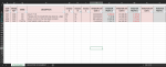
I have an investor spreadsheet with products [vehicles] that have been sold and their profits. call this stocksheet

Some vehicles have multiple investors (maximum 3 investors) on the stocksheet.

I have created a seperate summary sheet per investor, called investor statement.

On investor statement, cells E4 F4 AND I4 self populate with vlookup once I manually enter vehicle cost code. In this example its W17.

I desperately need a formula for cells G4 and H4 to self populate when I enter W17 into D4.

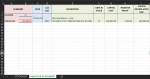
I would like G4 and H4 to firstly recognise D4 cost code W17 which was manually entered, then look at the investor name in B2, in this case YC, then lookup YC in stocksheet W17 and populate itself from the range T19 to Y19.

the tricky part for me is that it needs to recognise which cell investor YC is in the stocksheet for that cost code W17.

If he is investor A, B, or C it needs to return the correct values accordingly from the range T19 to Y19.

I fiddled with vlookup and match but couldnt get it right.

Please assist. much appreciated


thanks in advance.

Nazir

 

[cyrilbrd]

Hi, re investor statement, a good habit would be to enter data in a single row... Wrap text and Merge and center or unaligned data are a bit more tricky to handle.
Example date is row 3 cost code is row 4.

 

[KRice]

Welcome to the MrExcel board, Nazir.

Try this to see if it gives the results you were expecting. I've added YC as both investor A and C in this example to confirm that the formulas were pulling information from the right columns in the STOCKSHEET.

Book1.xlsx
	A	B	C	D	E	F	G	H	I	J	K	L	M	N	O	P	Q	R	S	T	U	V	W	X	Y
1
2			Cost Code	Model Year	Make	Description	Investor A	Investor B	Investor C											Investor Cap Cost A	Investor Profit A	Investor Cap Cost B	Investor Profit B	Investor Cap Cost C	Investor Profit C
3			W19	2018	VW	GOLF 1	MG	NC												300000	3398	210000	2379
4			W17	2018	VW	TIGUAN	YC	IH	YC											301000	7118	140000	3321	13000	1111
5			W20	2019	VW	GOLF 2	IH	YC												308000	3830	143000	1779
6			W21	2019	Toyota	FORTUNER	YC	IH												196000	1924	360000	3535
STOCKSHEET

Book1.xlsx
	A	B	C	D	E	F	G	H	I
1	SUMMARY		DATE	cost code	DESCRIPTION	DAYS IN STOCK	CAPITAL COST	INVESTOR PROFIT	CAPITAL RETURN AFTER SALE
2	INVESTOR	YC	10-Feb-19
3
4	CAPITAL INV	350000		W17	TIGUAN	75	314000	8229	300000
5
INVESTOR STATEMENT

Cell Formulas
Range	Formula
G4	G4	=SUMPRODUCT(--(STOCKSHEET!$G$3:$G$6=$B$2),--(STOCKSHEET!$C$3:$C$6=$D4),INDEX(STOCKSHEET!$C$3:$Y$6,,18)) + SUMPRODUCT(--(STOCKSHEET!$H$3:$H$6=$B$2),--(STOCKSHEET!$C$3:$C$6=$D4),INDEX(STOCKSHEET!$C$3:$Y$6,,20)) + SUMPRODUCT(--(STOCKSHEET!$I$3:$I$6=$B$2),--(STOCKSHEET!$C$3:$C$6=$D4),INDEX(STOCKSHEET!$C$3:$Y$6,,22))
H4	H4	=SUMPRODUCT(--(STOCKSHEET!$G$3:$G$6=$B$2),--(STOCKSHEET!$C$3:$C$6=$D4),INDEX(STOCKSHEET!$C$3:$Y$6,,19)) + SUMPRODUCT(--(STOCKSHEET!$H$3:$H$6=$B$2),--(STOCKSHEET!$C$3:$C$6=$D4),INDEX(STOCKSHEET!$C$3:$Y$6,,21)) + SUMPRODUCT(--(STOCKSHEET!$I$3:$I$6=$B$2),--(STOCKSHEET!$C$3:$C$6=$D4),INDEX(STOCKSHEET!$C$3:$Y$6,,23))

 

[faqir41]

thanks a lot krice!! you are a legend! your formula worked perfectly! much appreciated.

@cyrilbrd...thanks for the guideline. the spreadsheet has more columns that are hidden due to me not wanting to complicate the question. so all good. thanks.

 

[KRice]

That's good news. Glad to help.