Copy entire row to matching sheet name (Macro)

[ifeelalone]

How can you copy an entire row to its matching sheet name based on cell value?

Main Sheet: criteria is in column B where the value and its entire row shall be copied to its matching sheet name

Here's the sheet names
1.

2.

3.

 

[Peter_SSs]

For the future, I'd also suggest that you look at the link in my signature block below for providing sample data. You will get many more potential helpers if they can copy the sample data to their worksheets rather than having to type it out from an image.

.. and also many helpers choose not to download files from other sites or, due to security restrictions at their work sites, are unable to download such files.

 

[ifeelalone]

I'm very sorry Mr. Peter. I'll recreate my question again for easy understanding. I'm really sorry to all. Thank you for educating me those tricks on how to post easily

 

[Peter_SSs]

I'm very sorry Mr. Peter. I'll recreate my question again for easy understanding. I'm really sorry to all. Thank you for educating me those tricks on how to post easily

You don't need to apologise but the easier you can make it for helpers, the more likely you are to get help.
So if possible, just post here again with a small set of data (change any sensitive bits) from the Summary sheet that we can copy to test with.

 

[ifeelalone]

Hey guys, this is a report to further simplify the table I am asking for help

I'm doing another file with the same goal - Copy entire row to matching sheet name,
but now, the column C is now my reference and matching sheet name. and I'm given an error with this.

Excel 2016 (Windows) 32 bit

	A​	B​	C​	D​	E​	F​	G​	H​	I​	J​	K​	L​	M​
1​						Deposits ​					Amount Posted ​
2​		Deposit Date​	SK Partner/Client/chk#​	Lot#​	CHECK No.​	BOA(Cash) ​	BOA(Check) ​	Citibank/BOA Teller/Wire ​	CREDIT CARD ​	Total (BOA & Citi) ​	Cash ​	Check ​	Total Amount Posted in GOMS ​
3​		01/05/16​	Andy Carpio		1670​		12,388.00​			26,823.00 ​		12,388.00​	26,823.00 ​
4​		01/05/16​	Art Tesnado	lot 1​	1671​		13,213.00​			14,435.00 ​		13,213.00​	14,435.00 ​
5​		01/05/16​	Alvin Empleo		1335​		1,222.00​			1,222.00 ​		1,222.00​	1,222.00 ​
6​										0.00 ​			0.00 ​
7​

<tbody>
</tbody>

Sheet: Summary

<tbody>
</tbody>

Kindly take note that the column C is a dropdown list (Data Validation-List) type and the whole table was formatted as table.

This is the code that I am using, can you tell me what is wrong?
I am using the code of Mr. Peter.

Sub MoveToSheets()

For Each ws In Worksheets
If ws.Name <> "Summary" Then
ws.UsedRange.Clear
Sheets("Summary").UsedRange.Copy Destination:=ws.Range("A1")
With ws.UsedRange
.AutoFilter Field:=3, Criteria1:="<>" & ws.Name, Operator:=xlAnd, Criteria2:="<>"
.Offset(1).EntireRow.Delete
.AutoFilter
End With
End If
Next ws
End Sub

Thank you for your help.

 

[Peter_SSs]

Thanks for providing sample data that is easy to copy & use.

You have a few things making this a bit different from the original problem.

1. Column A is blank so your used range probably doesn't start in column 1.

2. Your headings are in row 2 whereas they were in row 1 in the original problem.

3. Your data is a 'table' which already has its own filters built in.

See if this version does what you want.

[color=darkblue]Sub[/color] MoveToSheets_v2()
  [color=darkblue]Dim[/color] ws [color=darkblue]As[/color] Worksheet
  [color=darkblue]Dim[/color] lr [color=darkblue]As[/color] [color=darkblue]Long[/color]
  
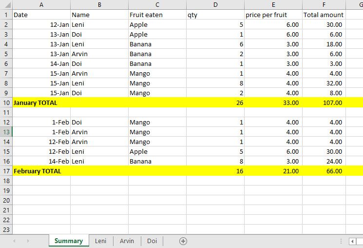
  [color=darkblue]With[/color] Sheets("Summary")
    lr = .Cells.Find(What:="*", After:=.Cells(1, 1), LookIn:=xlValues, SearchOrder:=xlByRows, SearchDirection:=xlPrevious, SearchFormat:=False).Row
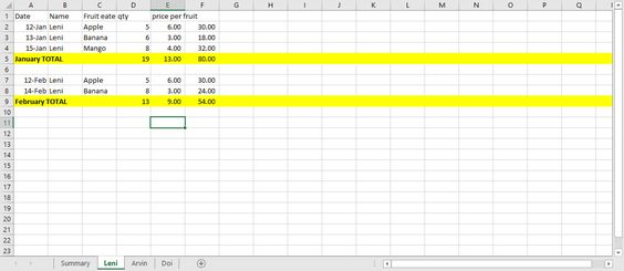
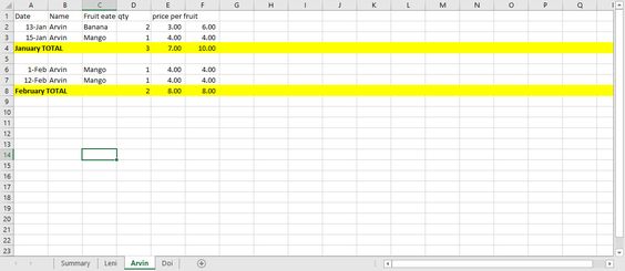
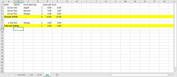
    For [color=darkblue]Each[/color] ws [color=darkblue]In[/color] Worksheets
      [color=darkblue]If[/color] ws.Name <> .Name [color=darkblue]Then[/color]
        ws.UsedRange.Clear
        .Rows(1).Resize(lr).Copy Destination:=ws.Range("A1")
        [color=darkblue]With[/color] ws.ListObjects(1).Range
          .AutoFilter Field:=2, Criteria1:="<>" & ws.Name
          .Offset(1).EntireRow.Delete
          .AutoFilter
        [color=darkblue]End[/color] [color=darkblue]With[/color]
      [color=darkblue]End[/color] [color=darkblue]If[/color]
    [color=darkblue]Next[/color] ws
  [color=darkblue]End[/color] [color=darkblue]With[/color]
[color=darkblue]End[/color] [color=darkblue]Sub[/color]

 

[ifeelalone]

Thanks it worked perfectly! but how can you exclude a sheet from the loop? I have "Reference_List" sheet where I put all the reference of my data validation-list. How would you exclude that sheeT?

 

[Peter_SSs]

but how can you exclude a sheet from the loop? I have "Reference_List" sheet where I put all the reference of my data validation-list. How would you exclude that sheeT?

The same way that we excluded the Summary sheet

If ws.Name <> .Name And ws.Name <> "Reference_List" Then

 

[ifeelalone]

Thank you Mr. Peter!

 

[Kriimu]

This code is wonderful, but how can i change it so that it does not delete other information from those tabs?