Applying an Excel formula in VBA

[SilverBirch]

Hello guys,

I need your help.
My created a long formula in Excel and I need to convert it to VBA. I've been trying a couple of things, but always failed. Can you please help me?

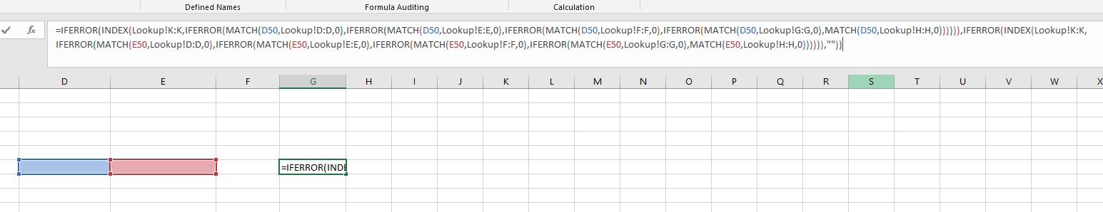
So the formula (for example for cell G50) looks like this:

=IFERROR(INDEX(Lookup!K:K,IFERROR(MATCH(D50,Lookup!D:D,0),IFERROR(MATCH(D50,Lookup!E:E,0),IFERROR(MATCH(D50,Lookup!F:F,0),IFERROR(MATCH(D50,Lookup!G:G,0),MATCH(D50,Lookup!H:H,0)))))),IFERROR(INDEX(Lookup!K:K,IFERROR(MATCH(E50,Lookup!D:D,0),IFERROR(MATCH(E50,Lookup!E:E,0),IFERROR(MATCH(E50,Lookup!F:F,0),IFERROR(MATCH(E50,Lookup!G:G,0),MATCH(E50,Lookup!H:H,0)))))),""))

Lookup is the name of another sheet.
I tried something like this, but with no result

theCell.FormulaR1C1 = "=IFERROR(INDEX(Lookup!K:K,IFERROR(MATCH(R[0]C[-3],Lookup!D:D,0),IFERROR(MATCH(R[0]C[-3],Lookup!E:E,0),IFERROR(MATCH(R[0]C[-3],Lookup!F:F,0),IFERROR(MATCH(R[0]C[-3],Lookup!G:G,0),MATCH(R[0]C[-3],Lookup!H:H,0)))))),IFERROR(INDEX(Lookup!K:K,IFERROR(MATCH(R[0]C[-2],Lookup!D:D,0),IFERROR(MATCH(R[0]C[-2],Lookup!E:E,0),IFERROR(MATCH(R[0]C[-2],Lookup!F:F,0),IFERROR(MATCH(R[0]C[-2],Lookup!G:G,0),MATCH(R[0]C[-2],Lookup!H:H,0)))))),""))"

Help me, please!

 

[steve the fish]

Hi. Do you know how to use the macro recorder? Record putting the formula into the cell and you will have your code. Your code fails because you are mixing the two reference styles which you cant do. You cant use A1 style, eg K:K, with RC style, eg R[0]C[-3].

 

[SilverBirch]

Hmm, I've unified the styles, but it doesn't work still.

I get "Application-defined or object defined-error".

Sub myTest()

Dim sh As Worksheet
Dim i As Integer
Dim c As Range
    
    Set sh = ActiveSheet
    
    For i = 2 To 35
        Set c = sh.Cells(i, 7)
        c.FormulaR1C1 = "=IFERROR(INDEX(Lookup!C[4],IFERROR(MATCH(R[0]C[-3],Lookup!C[-3],0),IFERROR(MATCH(R[0]C[-3],Lookup!C[-2],0),IFERROR(MATCH(R[0]C[-3],Lookup!C[-1],0),IFERROR(MATCH(R[0]C[-3],Lookup!C,0),MATCH(R[0]C[-3],Lookup!C[1],0)))))),IFERROR(INDEX(Lookup!C[4],IFERROR(MATCH(R[0]C[-2],Lookup!C[-3],0),IFERROR(MATCH(R[0]C[-2],Lookup!C[-2],0),IFERROR(MATCH(R[0]C[-2],Lookup!C[-1],0),IFERROR(MATCH(R[0]C[-2],Lookup!C,0),MATCH(R[0]C[-2],Lookup!C[1],0)))))),""))"
    Next i


End Sub

 

[steve the fish]

At the end of your formula for the IFERROR value if error you have "", change it to """".

 

[SilverBirch]

Yes, it works now!
Thank you Steve, you're the man! (or the fish!)