Automatic Highlighting of nearest values based on one manually highlighted cell's value

[jsk123]

Please take a look at this image.

This spreadsheet contains a separate continuous sequence of numbers. Each sequence is present in a separate column and is completely independent from the other sequences.
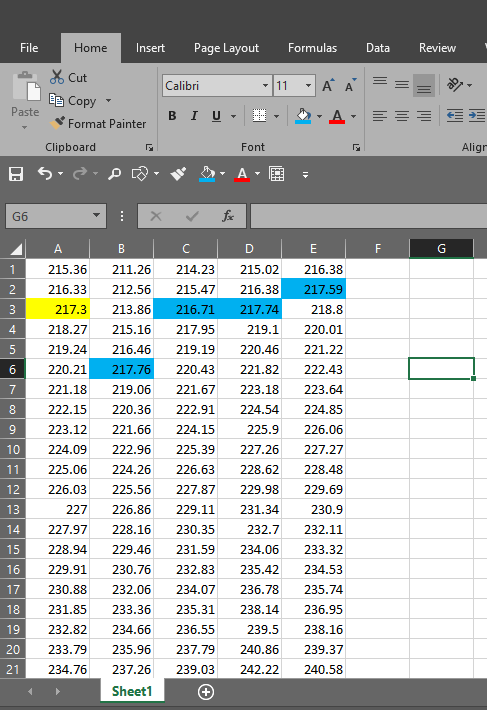
What I will do is... I will highlight a value in the first column in yellow.
What I want Excel to do is... It should highlight the cells values (in blue) in remaining columns that are closest to the cell's value I highlighted in yellow

For example, please take a look at the image...
I highlighted 217.3 in Column A in Yellow. Now, In the remaining columns, B,C,D and E, the cells with closest value to 217.3 must be highlighted in e.g. Blue by excel .

How to achieve this? I want this to be able to dynamically update the sheet when I remove the highlight or add new highlights...

Please guide me...

 

[Eric W]

As MAIT said before, there is no event trigger that fires when you manually change the color of a cell. The same is true of Conditional Formatting. It can't "see" if a cell is highlighted or not. If you want to use CF only, with no VBA, the best suggestion I can offer would be to enter the value of interest in another cell, for example G1. Given your example above, you'd put 217.3 in G1. Then follow these steps:

1) Select column A
2) Click Conditional Formatting > New Rule > Use a Formula > and enter:
=AND(A1=$G$1,A1<>"")
3) Select a yellow fill color and click OK.

4) Select columns B:E
5) Click Condiational Formatting > New Rule > Use a Formula > and enter:
=AND(B1<>"",ABS(B1-$G$1)=MIN(ABS(B$1:B$100-$G$1)))
6) Select a blue fill color and click OK.

The 100 in the formula refers to the bottom row of your data, just pick something equal to or below the last line of data, but not too huge since it will affect performance.

Now when you change G1 the colors will change to match. If this is not workable for you, then I can talk you through the other option I mentioned. This would be a VBA event handler where you would double click a cell in column A, and it would highlight the matching cells for you. But these are about the only 2 methods I can think of.

Let us know if this works for you.

 

[jsk123]

Thank you so much @EricW I like this solution.... Added a few customizations and it is ok ok... good enough to get the job done...