Hello,
I'm hoping someone can solve this very complicated problem I'm having with an Excel Sheet.
I have a table that is occupied by cells that represent 3 colors combined with letters. In other words...I created dropdown lists for every cell that offers just 3 options. (R Y and G)
I created colors to fill the cells based on the letter they choose. R=Red. Y=Yellow and G=Green. All good there. People love just using dropdowns to fill the cells.
I have a row at the bottom that is supposed to figure out averages from the individual columns above.
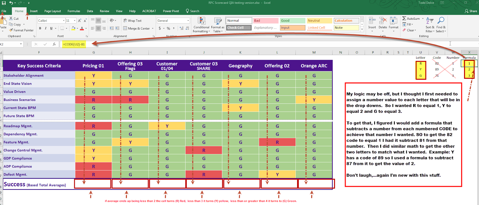
Obviously its not logical to write a formula that knows how to average colors or letters so I associated number values to each letter. R=1, Y=2 and G=3. I have 3 separate formulas for each of those associations.
I think I created them correctly.
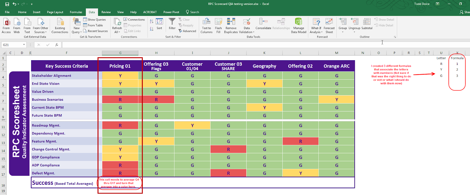
Now I'm stumped! How do I tell the bottom cell in column G to average the total values of all of the above cells in that same column based on my formulas?
In this example...I would need cell G18 to be able to add, then average the total of G4 thru G17 and use my 3 formulas that explain the numerical values of each letter in those cells. I will then need each bottom cell to do the same for their respective columns as well once I can figure out what to enter in the cell.
Thanks so much to anyone that may be able to walk me through this.
I'm hoping someone can solve this very complicated problem I'm having with an Excel Sheet.
I have a table that is occupied by cells that represent 3 colors combined with letters. In other words...I created dropdown lists for every cell that offers just 3 options. (R Y and G)
I created colors to fill the cells based on the letter they choose. R=Red. Y=Yellow and G=Green. All good there. People love just using dropdowns to fill the cells.
I have a row at the bottom that is supposed to figure out averages from the individual columns above.
Obviously its not logical to write a formula that knows how to average colors or letters so I associated number values to each letter. R=1, Y=2 and G=3. I have 3 separate formulas for each of those associations.
I think I created them correctly.
Now I'm stumped! How do I tell the bottom cell in column G to average the total values of all of the above cells in that same column based on my formulas?
In this example...I would need cell G18 to be able to add, then average the total of G4 thru G17 and use my 3 formulas that explain the numerical values of each letter in those cells. I will then need each bottom cell to do the same for their respective columns as well once I can figure out what to enter in the cell.
Thanks so much to anyone that may be able to walk me through this.