Basing calculations on cell colours - possible?

billv84

New Member
Joined
Mar 11, 2023
Messages
8
Office Version
  1. 365
Platform
  1. Windows
Hi all,

Hoping someone with a more powerful brain than me can help solve this problem!

I work in a school. We obviously record pupil progress in core subjects like maths and English in an MIS.
But for other subjects, something far simpler is acceptable.

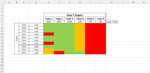
We are trying to come up with an Excel template where we can have a vertical list of pupil names, then a horizontal list of topics within a subject running across the top.
For each topic, every pupil with be RAG-rated (i.e. red-limited progress, amber-getting there, green-got it).
To reduce teacher workload, we could apply red and amber by exception - i.e. the default is green.

What I'd like to know is if it's possible to have a 'total'-style column, running horizontally underneath the row of topic headers, which will show a percentage (or something similar) to indicate how much of the class have met expectations for that topic (i.e. been graded as green).

I've attached an image with a rough idea of what I'm trying to explain.

Thank you very much in advance for any help!

Bill
 

Attachments

  • Screenshot 2023-03-11 094405.png
    Screenshot 2023-03-11 094405.png
    22.6 KB · Views: 15

Excel Facts

Back into an answer in Excel
Use Data, What-If Analysis, Goal Seek to find the correct input cell value to reach a desired result
Hi,
With Excel ... EVERYTHING is possible !!! :)

What is the method which is adding your colors to your cells ?

Is it Manually ... or with some kind of a formula, using Conditional Formatting ?
 
Last edited:
Upvote 0
Hi,
With Excel ... EVERYTHING is possible !!! :)

What is the method which is adding your colors to your cells ?

Is it Manually ... or with some kind of a formula, using Conditional Formatting ?
Thanks for the reply! Erm...I guess just manually?
 
Upvote 0
OK ...
Could you give an example of what needs to be done for your Red cells ....
 
Upvote 0
OK ...
Could you give an example of what needs to be done for your Red cells ....
To be honest, in it's simplest form, we can sort of ignore the cells which are red or amber. It is enough (I think) for us to just know what percentage of the cells in each column are green (i.e. "Ok, so I know 85% of my class understood that topic [because 85% were graded 'green']...but I know our pre-agreed 'success' threshold was 95%, so I know I need to go back and re-teach some of that content, or arrange catch-up sessions with anyone I can see who is red or amber"

I guess the percentage total is just a quick, numeric ready-reckoner to record, based on a % number rather than just staring at a list of colours and using gut feel.

Hope that makes sense!
 
Upvote 0
To me, this would be much easier to calculate and just as easy to use if you used your RAG rating in the cell and had conditional formatting apply the colour rather than manually applying colour.

In the sample below, in the conditional formatting I have made the font a slightly different colour to the background so that you can see it but in your actual sheet once you have it working, make the font in the CF exactly the same colour as the background 'Fill' colour and it will look just like your sample.
Start by entering a g (or G) in all the cells (select all cells, type g and confirm all with Ctrl+Enter).
Then if you want to mark a student as amber or red, just type an a or r in the relevant cell.
As you can see, the formula for the % calculation is then pretty simple.

billv84.xlsm
DEFGHIJ
5Topic 1Topic 2Topic 3Topic 4Topic 5Topic 6
660%90%100%10%0%0%
7Lastgggarr
8Lastgggarr
9Lastgggarr
10Lastrggarr
11Lastgggarr
12Lastgggarr
13Lastrggarr
14Lastgggarr
15Lastaggarr
16Lastarggrr
Sheet1
Cell Formulas
RangeFormula
E6:J6E6=COUNTIF(E7:E16,"g")/COUNTA(E7:E16)
Cells with Conditional Formatting
CellConditionCell FormatStop If True
E7:J16Expression=E7="r"textNO
E7:J16Expression=E7="a"textNO
E7:J16Expression=E7="g"textNO
Peter - loving the pragmatism with this solution! Thank you so much for taking the time to come up with this suggestion. I'm going to have a play around with this shortly. Thanks again!
 
Upvote 0
Peter - loving the pragmatism with this solution! Thank you so much for taking the time to come up with this suggestion. I'm going to have a play around with this shortly. Thanks again!
Hope it works for you but if there are any issues post back with the details.
 
Upvote 0

Forum statistics

Threads
1,215,232
Messages
6,123,759
Members
449,120
Latest member
Aa2

We've detected that you are using an adblocker.

We have a great community of people providing Excel help here, but the hosting costs are enormous. You can help keep this site running by allowing ads on MrExcel.com.
Allow Ads at MrExcel

Which adblocker are you using?

Disable AdBlock

Follow these easy steps to disable AdBlock

1)Click on the icon in the browser’s toolbar.
2)Click on the icon in the browser’s toolbar.
2)Click on the "Pause on this site" option.
Go back

Disable AdBlock Plus

Follow these easy steps to disable AdBlock Plus

1)Click on the icon in the browser’s toolbar.
2)Click on the toggle to disable it for "mrexcel.com".
Go back

Disable uBlock Origin

Follow these easy steps to disable uBlock Origin

1)Click on the icon in the browser’s toolbar.
2)Click on the "Power" button.
3)Click on the "Refresh" button.
Go back

Disable uBlock

Follow these easy steps to disable uBlock

1)Click on the icon in the browser’s toolbar.
2)Click on the "Power" button.
3)Click on the "Refresh" button.
Go back
Back
Top