Compare numbers

[mallee]

Hi guys,

I found myself chasing my own tail at work, and could use some extra input. I'm basically just trying to compare to columns with a condition.

There are two variables:
- Buildings - 3 to 5 alphanumeric code in a format of 3 or 4 digits, or 3 digits followed by a single letter, or 4 digits by a single letter. These codes are unique.
- Business - 4 digit code only. These codes are NOT unique, and same code can be attached to all the Buildings.

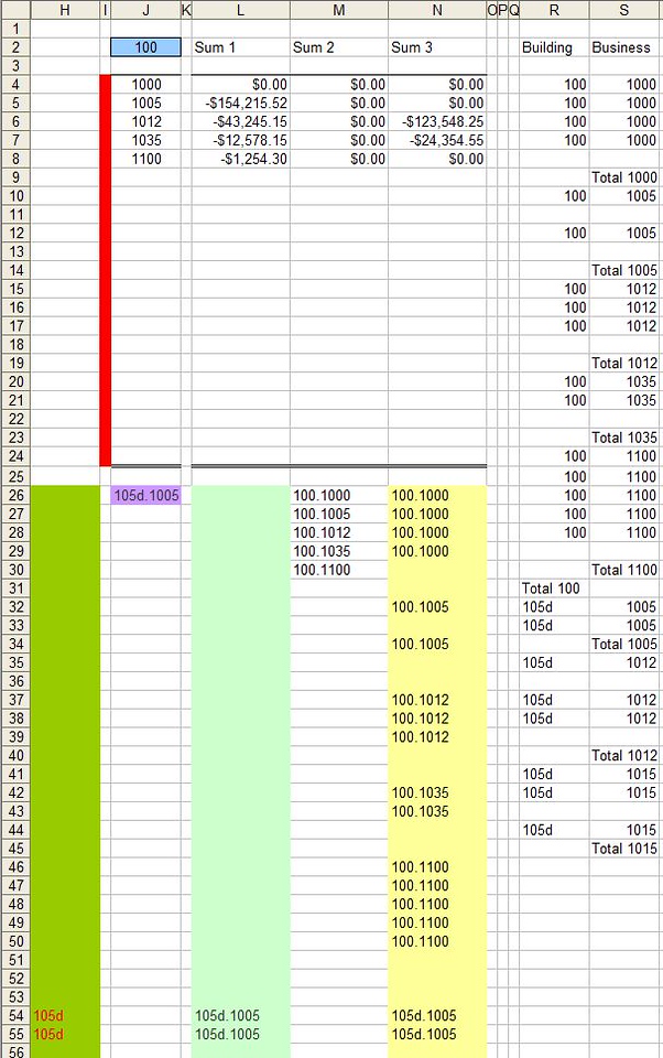
J2 - that's my drop down menu option for Buildings (table links back to another sheet)
J4:J24 - Business codes pulled from another sheet based on J2 selection (max of 20 businesses)

L4:K24 - sumifs pulling from the report in R4:Z1000

Goal: Upon selecting a Building from J2 drop down, I want a cell to show me a missing Business (if any) is listed in the report R4:Z1000 that's not in J4:J24.

What I've done so far, before finally throwing a towel, I combined the Building and Business numbers together in Col-N

=IF(OR(R18="",S18=""),"",<wbr style="font-family: arial, sans-serif; font-size: 12.8px;">CONCATENATE(R18,".",S18))

In Col-M I'm just pointing back to the list of business with an IF statement.

Col-L, I'm comparing codes between the two with:

=IF(ISERROR(VLOOKUP(N27,$M$27:<wbr style="font-family: arial, sans-serif; font-size: 12.8px;">$M$43,1,FALSE)),N27,"")

And then in Col-J, I wanted to list the first non-zero entry

=INDEX(L27:L500,MATCH(TRUE,<wbr style="font-family: arial, sans-serif; font-size: 12.8px;">INDEX(L27:L500<>"",),0))

But that only works if my report is for a single building only, which doesn't help me at all.

I then added extracted the Building code from Col-J with

=IF(L27<>"",LEFT(L27,(FIND("."<wbr style="font-family: arial, sans-serif; font-size: 12.8px;">,L27,1)-1)),"")

And tried to compare that to J2, and link back to Col-N to find the missing Business, but I found myself in way over my head with this.

There's got to be an easier way to get it done. I hope

 

[mallee]

OK, so in the cell J26 I replaced the current formula with:

=LOOKUP(1E+100,SEARCH(J2,L26:L500),L27:L500)

And that almost works. It works if my building selection in J2 is completely unique, but when I'm faced with building coeds such as '100' and '100A' in the report, the value in J26 will return an entry that matches '100A' despite having selected '100' in J2.

Is there a way to format the above formula, so that it only looks up the partial string value before the period?

 

[mallee]

Figured it out.

Added =CONCATENATE(J2,".") in I2, and referenced that instead of J2 in the above =LOOKUP formula.

Next, I reference J26 with =IFNA() and seems to work now as intended.