Counting the number of rows that meet multiple criteria

D-Angle

New Member
Joined
Aug 24, 2011
Messages
23
Hello all :)

I'm a long-time reader of these boards, they have given me a lot of help and tips in the past and kept me in a job on more than one occasion. :) I'm now stuck on a spreadsheet in which I am trying to analyse a large amount of data using formulas, and none of the suggested solutions I have found seem to work. This is a section of the dataset I am working on, it's a sheet of hourly prices of the FTSE100 Index:
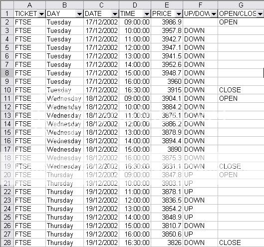
FTSEsheet.jpg


What I would like to do, is count the number of rows that meet the same criteria in multiple cells. For example, I would like to count how many times the index was up at 3pm on a Wednesday, how many times it opened down on a Tuesday etc. I would also like to get more complex results as well, such as how many times the index was, say, up at 3pm when it was down at 10am, which I think would be easier to generate if I could count how many rows met those 2 criteria to start with. Most of my searching suggested DCOUNTA, but nothing seems to give a valid result.

Any suggestions greatly appreciated!
 
Btw you are correct that "TRUE" is actually text.

You can test this by using the following formula pointed at one of your TRUE values:
=TRUE=A1

It should return FALSE if your values are text.

For the example of the formula working below I have replaced "True" with "Text" to avoid ambiguity.

Excel Workbook
ABCDEF
1texttexttexttext16
2text
3text
4text
5
6text
7
8texttext
9
10
11text
12
13
14text
15text
16
17text
18texttext
19
20text
21text
22text
23
24texttext
25
26text
Sheet1
 
Upvote 0

Excel Facts

How to fill five years of quarters?
Type 1Q-2023 in a cell. Grab the fill handle and drag down or right. After 4Q-2023, Excel will jump to 1Q-2024. Dash can be any character.
Hi guys,

I have a similar query but the formulae provided in this forum aren't working for my data. Essentially I want to count the number of rows that contain text 'True' in either of the 4 columns I have. I do not want the formula to count the row twice if that row which has the text 'True' is in column C as well as D.

I am using Excel Microsoft Office Professional 2010. Any help would be appreciated.

Control+shift+enter, not just enter:

=SUM(IF(MMULT((A2:D15=TRUE)+0,TRANSPOSE(COLUMN($A$2:$D$15)^0)),1))
 
Upvote 0
I used the test formula and it worked but when I use the formula below:

=SUMPRODUCT(--((A1:A8="TRUE")+(B2:B8="TRUE")+(C2:C8="TRUE")+(D2:D8="TRUE")>0))
it comes as #N/A

(sorry for some reason I couldn't printscreen and paste onto the forum

ABCD
1FalseFalseFalseFalse
2TrueTrueTrueTrue
3TrueTrueFalseFalse
4FalseFalseFalseFalse
5TrueTrueTrueTrue
6TrueTrueFalseFalse
7FalseFalseFalseFalse
8TrueFalseFalseFalse

<tbody>
</tbody>
 
Upvote 0
Hello Aladin,

The formula worked! Please can you explain how the formula is working so I can apply further. Thank you guys, you are legends in my book

Baseem
 
Upvote 0
Hi,

Using VBA I came up with the code below (4 columns, 100 rows):
Code:
i = 0
For Row = 1 To 100
j = 0
    For col = 1 To 4
        If Cells(Row, col).Value = "TEXT" Then
        j = j + 1
        End If
    Next col
    If j > 0 Then
        i = i + 1
    End If
Next Row


MsgBox ("results:" & i)

Can you guys suggest other alternatives? I'm new to VBA :D
 
Upvote 0
I used the test formula and it worked but when I use the formula below:

=SUMPRODUCT(--((A1:A8="TRUE")+(B2:B8="TRUE")+(C2:C8="TRUE")+(D2:D8="TRUE")>0))
it comes as #N/A

Stick with Aladin's but.. either:

=SUMPRODUCT(--((A2:A8="TRUE")+(B2:B8="TRUE")+(C2:C8="TRUE")+(D2:D8="TRUE")>0))

or

=SUMPRODUCT(--((A2:A8=TRUE)+(B2:B8=TRUE)+(C2:C8=TRUE)+(D2:D8=TRUE)>0))
 
Upvote 0
Hi FormR,

Thanks the latter of the two formulae worked as well!btw what is the difference between using the operator + and using * in excel and is this <> mean not equal to
 
Upvote 0
the latter of the two formulae worked as well!

Cool :) although this would indicate that the below statement was not technically true..

Btw you are correct that "TRUE" is actually text.

The plus operator in this instance is used as an OR statement versus the * which is used as an AND statement.

btw what is the difference between using the operator + and using * in excel and is this <> mean not equal to
 
Upvote 0
BTW - these can be tricky concepts and everything I know on the subject I learnt from hanging out at this forum de-ciphering solutions posted by the likes of Aladin.
 
Upvote 0
Hello Aladin,

The formula worked! Please can you explain how the formula is working so I can apply further. Thank you guys, you are legends in my book

Baseem

Given a part your previous exhibit in A2:D4 for ease of exposition...

FALSEFALSEFALSEFALSE
TRUETRUETRUETRUE
TRUETRUEFALSEFALSE

<COLGROUP><COL style="WIDTH: 48pt" span=4 width=64><TBODY>
</TBODY>

We have the following successive evalutions of the formula..

SUM(IF(MMULT(($A$2:$D$4=TRUE)+0,TRANSPOSE(COLUMN($A$2:$D$4)^0)),1))

==> (the semi-colon means: per row)

SUM(IF(MMULT(({FALSE,FALSE,FALSE,FALSE;TRUE,TRUE,TRUE,TRUE;TRUE,TRUE,FALSE,FALSE}=TRUE)+0,TRANSPOSE(COLUMN($A$2:$D$4)^0)),1))

==> (TRUE=TRUE yields TRUE, otherwise FALSE)

lSUM(IF(MMULT(({FALSE,FALSE,FALSE,FALSE;TRUE,TRUE,TRUE,TRUE;TRUE,TRUE,FALSE,FALSE})+0,TRANSPOSE(COLUMN($A$2:$D$4)^0)),1))

==> (adding a 0 to a TRUE yields 1; adding a 0 to a FALSE yields 0)

SUM(IF(MMULT({0,0,0,0;1,1,1,1;1,1,0,0},TRANSPOSE(COLUMN($A$2:$D$4)^0)),1))

==> (the column bit)

SUM(IF(MMULT({0,0,0,0;1,1,1,1;1,1,0,0},TRANSPOSE({1,2,3,4}^0)),1))

==> (the column bit raised to the power 0 yields an horizontal identity vector)

SUM(IF(MMULT({0,0,0,0;1,1,1,1;1,1,0,0},TRANSPOSE({1,1,1,1})),1))

==> (transposing the horizontal vector yields a vertical identity vector)

SUM(IF(MMULT({0,0,0,0;1,1,1,1;1,1,0,0},{1;1;1;1}),1))

==> (note that MMULT will multiply a matrix with an appropriate identity vector)

SUM(IF({0;4;2},1))

==> (IF considers a zero value as FALSE, a non-zero value as TRUE)

SUM({FALSE;1;1})

==> (summing the 1's for non-zero values IF returns we get...)

2

which is the desired value.

To recap: We look for equality to TRUE per row, convert the evaluations into 1/0's, and feed them to MMULT as a matrix of which each row gets multiplied with a vertical identity vector. Such fed to an IF allows us to obtain a count. Note that this formula is easily extendible to more rows and columns.

Hope this helps.
 
Upvote 0

Forum statistics

Threads
1,215,506
Messages
6,125,189
Members
449,213
Latest member
Kirbito

We've detected that you are using an adblocker.

We have a great community of people providing Excel help here, but the hosting costs are enormous. You can help keep this site running by allowing ads on MrExcel.com.
Allow Ads at MrExcel

Which adblocker are you using?

Disable AdBlock

Follow these easy steps to disable AdBlock

1)Click on the icon in the browser’s toolbar.
2)Click on the icon in the browser’s toolbar.
2)Click on the "Pause on this site" option.
Go back

Disable AdBlock Plus

Follow these easy steps to disable AdBlock Plus

1)Click on the icon in the browser’s toolbar.
2)Click on the toggle to disable it for "mrexcel.com".
Go back

Disable uBlock Origin

Follow these easy steps to disable uBlock Origin

1)Click on the icon in the browser’s toolbar.
2)Click on the "Power" button.
3)Click on the "Refresh" button.
Go back

Disable uBlock

Follow these easy steps to disable uBlock

1)Click on the icon in the browser’s toolbar.
2)Click on the "Power" button.
3)Click on the "Refresh" button.
Go back
Back
Top