Counting the number of rows that meet multiple criteria

[D-Angle]

Hello all

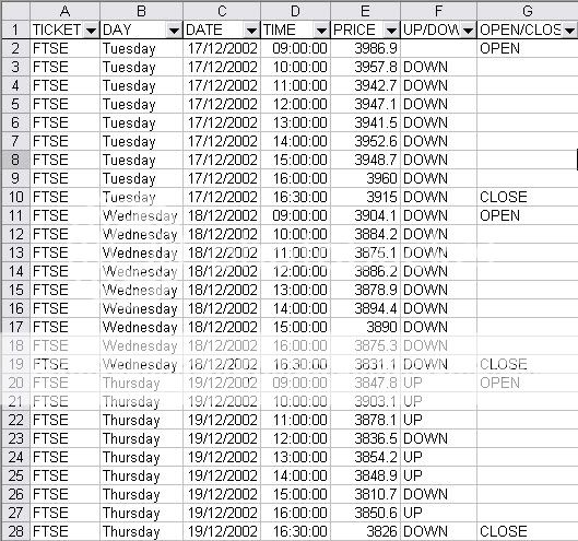
I'm a long-time reader of these boards, they have given me a lot of help and tips in the past and kept me in a job on more than one occasion. I'm now stuck on a spreadsheet in which I am trying to analyse a large amount of data using formulas, and none of the suggested solutions I have found seem to work. This is a section of the dataset I am working on, it's a sheet of hourly prices of the FTSE100 Index:

What I would like to do, is count the number of rows that meet the same criteria in multiple cells. For example, I would like to count how many times the index was up at 3pm on a Wednesday, how many times it opened down on a Tuesday etc. I would also like to get more complex results as well, such as how many times the index was, say, up at 3pm when it was down at 10am, which I think would be easier to generate if I could count how many rows met those 2 criteria to start with. Most of my searching suggested DCOUNTA, but nothing seems to give a valid result.

Any suggestions greatly appreciated!

 

[markmzz]

Try this too (with the layout of the post #13):

Use Enter to enter the formula

=SUM(SIGN(MMULT(--($A$1:$D$8=TRUE),ROW(INDIRECT("1:"&COLUMNS($A$1:$D$1))))))

Or this small modification in [COLOR=#0000ff]Aladin's formula [/COLOR]- use Ctrl+Shift+Enter to enter the formula

=SUM(SIGN(MMULT(--($A$1:$D$8=TRUE),TRANSPOSE(COLUMN($A$1:$D$1)))))

Markmzz

 

[Aladin Akyurek]

My formula needs no modification at all, especially not an additional function call. And I would never opt for convoluted, expensive formulas, if I can or when there is an alternative available.

 

[markmzz]

Sorry about that.

Use Ctrl+Shift+Enter to enter the formula

=SUM(SIGN(MMULT(--($A$1:$D$8=TRUE),TRANSPOSE(COLUMN($A$1:$D$1)))))

Markmzz

 

[Baseem]

Hi guys,

I have been using countif function for a column to find out number of rows which have the text 'Female' or 'Male'. However when I use the excel filter function and then manually highlight to count the total sum of rows which contain the above text the excel gives different numbers. Any reason for this, the only thing I can think of is that my formula is not correct or my data column is missing some text, ( I have been through them and cannot find any empty or different text to male/female.

My formula:=COUNTIF(D2:D580,"Male")

Hope I can once again seek the excel power of you legends. Cheers.

Baseem

 

[markmzz]

Hi guys,

I have been using countif function for a column to find out number of rows which have the text 'Female' or 'Male'. However when I use the excel filter function and then manually highlight to count the total sum of rows which contain the above text the excel gives different numbers. Any reason for this, the only thing I can think of is that my formula is not correct or my data column is missing some text, ( I have been through them and cannot find any empty or different text to male/female.

My formula:=COUNTIF(D2:D580,"Male")

Hope I can once again seek the excel power of you legends. Cheers.

Baseem

If I understand correctly what you want, maybe this can helps:

=SUMPRODUCT(($D$2:$D$580={"Male","Female"})*SUBTOTAL(3,OFFSET($D$2,ROW($D$2:$D$580)-ROW($D$2),)))

Markmzz

 

[Aladin Akyurek]

Hi guys,

I have been using countif function for a column to find out number of rows which have the text 'Female' or 'Male'. However when I use the excel filter function and then manually highlight to count the total sum of rows which contain the above text the excel gives different numbers. Any reason for this, the only thing I can think of is that my formula is not correct or my data column is missing some text, ( I have been through them and cannot find any empty or different text to male/female.

My formula:=COUNTIF(D2:D580,"Male")

Hope I can once again seek the excel power of you legends. Cheers.

Baseem

Conditional count under autofilter...

=SUMPRODUCT(
  SUBTOTAL(3,OFFSET(D2,ROW(D2:D580)-ROW(D2),0,1)),
  --(D2:D580="Male"))

If you want to count either male or female at the same time:

=SUMPRODUCT(
  SUBTOTAL(3,OFFSET(D2,ROW(D2:D580)-ROW(D2),0,1)),
  --ISNUMBER(MATCH(D2:D580,{"Male","Female"},0)))

 

[Gesyca_is_joy]

I have a slightly different variation on the same basic question. i am using Excel 2007. What I have is a very large table named "dataset" on one tab and on another I am trying to write a formula to count the number of cells that meet three variables. I want to write a formula that counts the number of cells that have "RM", "STCH" and "Open" in their columns. I know Excel allows me to use column headers and the table name in the formula so I tried to write a COUNTIFS function, I also tried a SUMPRODUCT although I am not as familiar with that one, and I keep getting the answer of 0. for instance in the snapshot below the answer would be 1. Can someone assist me?

Order Type	Site	Backlog Week 1
RM	STCH	Open
CM	STCH	Open
RM	WCK	CANCELLED
RM	STCH
CM	WCK	Open

<tbody>
</tbody>

 

[Aladin Akyurek]

I have a slightly different variation on the same basic question. i am using Excel 2007. What I have is a very large table named "dataset" on one tab and on another I am trying to write a formula to count the number of cells that meet three variables. I want to write a formula that counts the number of cells that have "RM", "STCH" and "Open" in their columns. I know Excel allows me to use column headers and the table name in the formula so I tried to write a COUNTIFS function, I also tried a SUMPRODUCT although I am not as familiar with that one, and I keep getting the answer of 0. for instance in the snapshot below the answer would be 1. Can someone assist me?

Order Type	Site	Backlog Week 1
RM	STCH	Open
CM	STCH	Open
RM	WCK	CANCELLED
RM	STCH
CM	WCK	Open

<TBODY>
</TBODY>

What are the conditions for the count you want? And what is the result you want to see for the sample you posted?

 

[markmzz]

I have a slightly different variation on the same basic question. i am using Excel 2007. What I have is a very large table named "dataset" on one tab and on another I am trying to write a formula to count the number of cells that meet three variables. I want to write a formula that counts the number of cells that have "RM", "STCH" and "Open" in their columns. I know Excel allows me to use column headers and the table name in the formula so I tried to write a COUNTIFS function, I also tried a SUMPRODUCT although I am not as familiar with that one, and I keep getting the answer of 0. for instance in the snapshot below the answer would be 1. Can someone assist me?

Order Type	Site	Backlog Week 1
RM	STCH	Open
CM	STCH	Open
RM	WCK	CANCELLED
RM	STCH
CM	WCK	Open

<tbody>
</tbody>

Try this:

=COUNTIFS(Table1[Order Type],"RM",Table1[Site],"STCH",Table1[Backlog Week 1],"Open")

Or

=SUMPRODUCT(-(Table1[Order Type]="RM"),-(Table1[Site]="STCH"),--(Table1[Backlog Week 1]="Open"))*
SUBTOTAL(3,OFFSET(Table1[[#Headers],[Order Type]],ROW(Table1[Order Type])-ROW(Table1[[#Headers],[Order Type]]),))

Markmzz

 

[Gesyca_is_joy]

Thank You! the COUNTIFS formula work a treat! Since i need this to be a formula that can be manipulated by the end user I entered a cell reference instead of "RM and "STCH", locked the sheet down except those two cells and gave the user a drop down option to select from. After troubleshooting against my live data it worked very well, thank you!