Data Table to Pivot Table then Update Data from Pivot Table

[jbesclapez]

Hello,

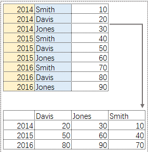
I would like to have a Data Table that creates a Pivot Table. Then I want to insert or change data in the pivot table that would "update" the Data Table back. It will be a 2 steps thing.

Here is the Table :

ColA	ColB	ColC	ColD
CH1.4	PE	Q001R19	OK
LOU	PE	Q001R13	ToDo
CH1.4	DIAR	Q001R22	OK
CH1.4	DIAR	Q001R31	OK
BID	LOCO	Q001R21	ToDo
BID	LOCO	Q001R31b	ToDo
CH1.4	LOCO	Q005R03	ToDo
GAP	OE	Q005R01	INCOH
CH1.4	OE	Q005R04	INCOH
CH1.4	OE	Q006R05	OK
GAP	OE	Q006R01	OK
BID	PE	Q001R19	OK
GAP	PE	Q001R13	ToDo
CH1.4	PE	Q005R04	OK
LOU	PE	Q001R31b	ToDo

<tbody>
</tbody>

And it creates a table like below (same then a pivot table)
Please note the cell A1. It has to be filtered on that which is the ColB of the table.

PE
	Q001R19	Q001R13	Q001R22	Q001R31	Q001R21	Q001R31b	Q005R03	Q005R01	Q005R04	Q006R05	Q006R01
CH1.4	OK								OK
LOU		ToDo				ToDo
BID	OK
GAP		ToDo

<tbody>
</tbody>

I know it is tricky because a Pivot table cannot be done as it does not work with Data. (only count, sum...). The trick I used was to put a unique number in ColD and in the pivot table show the MAX number. Then I did a replace to change the number with actual Name in ColD. However, I have not idea how to go back from Pivot Table to Data Table...

I hope one of you will know how to do that better than me.

Thanks for your time

 

[Fazza]

it isn't totally clear what is wanted

a query table can return the cross-tab table. like you describe, this can be done with a MAX (or other) function as it works on text

so a table such as

TRANSFORM MAX(ColD)
SELECT ColA
FROM YourTable
GROUP BY ColA
PIVOT ColC

And if you want it filtered, add
WHERE ColB = 'PE'
between the FROM and GROUP BY clauses

this could be parameterised and linked to a cell if it suited

I'll have a google for some old examples that are similar (in that they give the cross tab result), and post soon with link/s

PS here was one https://www.mrexcel.com/forum/excel-questions/384664-can-i-return-text-pivot-table.html

 

[jbesclapez]

Hi there,

Sorry for the late reply Fazza, but i got super busy and then the holidays came by... Now back to work. And I still have the same problem. This time I will try to describe it better with exemples.

Name	Color	Taste
John	Blue	Like
Pete	Blue	Dislike
Mike	Blue	Like
Frank	Blue	Dislike
John	Red	Like
Pete	Red	Dislike
John	Yellow	Like
Pete	Yellow	Dislike
Mike	Yellow	Like
Frank	Yellow	Dislike

<tbody>
</tbody>

This should turn into that :

	Blue	Red	Yellow
Frank	Dislike		Dislike
John	Like	Like	Like
Mike	Like		Like
Pete	Dislike	Dislike	Dislike

<tbody>
</tbody>

The source is always 3 columns.
The source is always in column F1 with a Header.
The Destination Should be in a worksheet called TabSI in cell A1
The source has N rows with no empty field.

In Kutools addin, it is under Range > Transpose Table Dimension > List to cross table.

Hope I am clearer now. Please could anyone help on that?


Thanks

 

[krrishkrsna]

got below formula from ExcelIsFun videos

place cursor in cell A1 and paste below data

Name	Color	Taste
John	Blue	Like
Pete	Blue	Dislike
Mike	Blue	Like
Frank	Blue	Dislike
John	Red	Like
Pete	Red	Dislike
John	Yellow	Like
Pete	Yellow	Dislike
Mike	Yellow	Like
Frank	Yellow	Dislike

<tbody>
</tbody>

type below formula in cell A14 and drag it down as many cells u wish, to list out unique names
=INDEX($A$2:$A$11,SMALL(IF(FREQUENCY(MATCH($A$2:$A$11,$A$2:$A$11,0),ROW($A$2:$A$11)-ROW($A$2)+1),ROW($A$2:$A$11)-ROW($A$2)+1),ROWS(A$14:A14)))

type below formula in cell B13 and drag it to right as many cells u wish, to list out unique color
=INDEX($B$2:$B$11,SMALL(IF(FREQUENCY(MATCH($B$2:$B$11,$B$2:$B$11,0),ROW($B$2:$B$11)-ROW($B$2)+1),ROW($B$2:$B$11)-ROW($B$2)+1),COLUMNS($B13:B13)))

type below formula in cell B14 and drag it to across the cells, to retrieve the column Taste values
=IFERROR(INDEX($C$2:$C$11,MATCH($A14&B$13,$A$2:$A$11&$B$2:$B$11,0)),"")

NOTE after typing complete formula press CTRL SHIFT ENTER to make array formula

hope it helps you

 

[jbesclapez]

got below formula from ExcelIsFun videos

place cursor in cell A1 and paste below data

Name	Color	Taste
John	Blue	Like
Pete	Blue	Dislike
Mike	Blue	Like
Frank	Blue	Dislike
John	Red	Like
Pete	Red	Dislike
John	Yellow	Like
Pete	Yellow	Dislike
Mike	Yellow	Like
Frank	Yellow	Dislike

<tbody>
</tbody>

type below formula in cell A14 and drag it down as many cells u wish, to list out unique names
=INDEX($A$2:$A$11,SMALL(IF(FREQUENCY(MATCH($A$2:$A$11,$A$2:$A$11,0),ROW($A$2:$A$11)-ROW($A$2)+1),ROW($A$2:$A$11)-ROW($A$2)+1),ROWS(A$14:A14)))

type below formula in cell B13 and drag it to right as many cells u wish, to list out unique color
=INDEX($B$2:$B$11,SMALL(IF(FREQUENCY(MATCH($B$2:$B$11,$B$2:$B$11,0),ROW($B$2:$B$11)-ROW($B$2)+1),ROW($B$2:$B$11)-ROW($B$2)+1),COLUMNS($B13:B13)))

type below formula in cell B14 and drag it to across the cells, to retrieve the column Taste values
=IFERROR(INDEX($C$2:$C$11,MATCH($A14&B$13,$A$2:$A$11&$B$2:$B$11,0)),"")

NOTE after typing complete formula press CTRL SHIFT ENTER to make array formula

hope it helps you

Hi Krrishhkrsna, I just tried that but it does not seem to be working.

	Blue	Blue	Blue
John
John
John
John

<tbody>
</tbody>

 

[jbesclapez]

My bad. I forgot to do the array. Now working.
Thanks

 

[jbesclapez]

Anyone would know how to do that in pure VBA?

 

[krrishkrsna]

create new workbook with .xlsm extension


follow the below link instructions
https://youtu.be/u-wvTDFbvw8



create new sheet and name as Formula
Distinct Count Name SUMPRODUCT(--(ISTEXT(NameRange))/COUNTIF(NameRange,NameRange&""))
Color SUMPRODUCT(--(ISTEXT(ColorRange))/COUNTIF(ColorRange,ColorRange&""))


Name Range OFFSET(Sheet1!$A$2,,,COUNTA(Sheet1!$A:$A)-1)
Color Range OFFSET(Sheet1!$B$2,,,COUNTA(Sheet1!$B:$B)-1)
Tast Range OFFSET(Sheet1!$C$2,,,COUNTA(Sheet1!$C:$C)-1)


uniqueName INDEX(NameRange,SMALL(IF(FREQUENCY(MATCH(NameRange,NameRange,0),ROW(NameRange)-ROW($A$2)+1),ROW(NameRange)-ROW($A$2)+1),ROWS(G$2:G2)))
uniqueColor INDEX(ColorRange,SMALL(IF(FREQUENCY(MATCH(ColorRange,ColorRange,0),ROW(ColorRange)-ROW($B$2)+1),ROW(ColorRange)-ROW($B$2)+1),COLUMNS($H1:H1)))
Tastedata IFERROR(INDEX(TasteRange,MATCH($G2&H$1,NameRange&ColorRange,0)),"")




create new sheet and name as Data
place cursor in range A1 and paste your raw data into that




press Alt F11 to open VBeditor window and paste below code into new module
Option Explicit


Sub PivotheunPivot()


Sheets("Data").Range("E1").FormulaArray = "=" & Sheets("Formula").Range("C1")
Sheets("Data").Range("E2").FormulaArray = "=" & Sheets("Formula").Range("C2")


'UniqueNameList
Sheets("Data").Range("G2").Select
ActiveCell.FormulaArray = "=" & Sheets("Formula").Range("C8")
ActiveCell.Offset(Range("E1") - 1, 0).Select 'E1 holding value of Name Distinct Count
Range(Selection, ActiveCell.End(xlUp)).Select
Selection.FillDown


'UniqueColorList
Sheets("Data").Range("H1").Select
ActiveCell.FormulaArray = "=" & Sheets("Formula").Range("C9")
ActiveCell.Offset(0, Range("E2") - 1).Select 'E2 holding value of Color Distinct Count
Range(Selection, Selection.End(xlToLeft)).Select
Selection.FillRight


'TasteResult
Sheets("Data").Range("H2").Select
ActiveCell.FormulaArray = "=" & Sheets("Formula").Range("C10")
Range(Selection, Selection.Offset(Range("E1") - 1, Range("E2") - 1)).Select
Selection.FillDown
Selection.FillRight


Range("A2").Select


End Sub




if you want to change sheet name Formula and Data, update changed name in VB code accordingly


i think this might helps you. i dont know how to upload excel file here so given lengthy instructions to you along with 6 min youtube video link :D

 

[Fazza]

For info, the solution I posted does what was asked. No formulas & no VBA. Also, it should be quick on large datasets.

TRANSFORM MAX(Taste)
SELECT Name
FROM YourTable
GROUP BY Name
PIVOT Color

 

[krrishkrsna]

hi Fazza,

is below SQL code and where needs to be enter

TRANSFORM MAX(Taste)
SELECT Name
FROM YourTable
GROUP BY Name
PIVOT Color[/QUOTE]