Find value according to different criteria and sum

[riskier4ra]

Hey there, anyone know how I can do the following? My guess is I would use Index Match but not sure how to involve the date aspect.

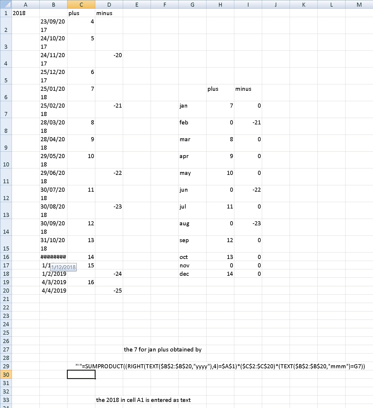
I need to sum some values that match by a common symbol under two different headings, but only if they fall within the same calendar year.

So. If sym A matches sym B check date for year and if the same sum the value of C1 & G1. If year in After does not match the year found in Before do nothing. Do not want to use SUMIF, would prefer to use SUMPRODUCT

Heading = Before
A1= Date
B1= Sym
C1= Numerical Value

Heading = After
E1= Date
F1= Sym
G1=Numerical Value

Thanks for any help you all can give,
Risk

 

[riskier4ra]

01/04/2018
	28/03/2018	3
	01/04/2018		-9
	05/04/2018	5					sum of pos
	09/04/2018		-8				60
	13/04/2018	22
	17/04/2018		-7
	21/04/2018	33
	25/04/2018		-6
	05/05/2018	44
	A1 is entered as a nomal date
	60 from
	=SUMPRODUCT((RIGHT(TEXT($B$2:$B$10,"mmm"),4)=TEXT($A$1,"mmm"))*($C$2:$C$10))
	it now sums for april
	if you wanted april 17 and april 18 more work is needed

<tbody>
</tbody>

No thats perfect thank you! Now if I could get you to show me what you did in the beginning to include the symbol, that would be golden!

 

[riskier4ra]

01/04/2018
	28/03/2018	3
	01/04/2018		-9
	05/04/2018	5					sum of pos
	09/04/2018		-8				60
	13/04/2018	22
	17/04/2018		-7
	21/04/2018	33
	25/04/2018		-6
	05/05/2018	44
	A1 is entered as a nomal date
	60 from
	=SUMPRODUCT((RIGHT(TEXT($B$2:$B$10,"mmm"),4)=TEXT($A$1,"mmm"))*($C$2:$C$10))
	it now sums for april
	if you wanted april 17 and april 18 more work is needed

<tbody>
</tbody>

Can I get it to pull the month data within what we have already developed?

For example: We now have the ability to find all values within a given year +/- and sum them (thanks to you!) and it works perfect. I would like to expand on it if possible and use the same structure, which according to my understanding, I would need to create 12 additional helper cells for each month with your sumproduct formula in each month, i.e C2:N2 that references the helper cell for the months but looks to the year selected in A1 to pull the sums from the available range of values. Is that possible?

=Changeable Year

=Helper Column

Jan

Feb

Mar

Apr

May

Jun

Jul

Aug

Sep

Oct

Nov

Dec

A1

Sums by year

Need a formula to allow me to sum all values for this month within the year selected

and this one

and this one

and this one

etc

etc

etc

etc

etc

etc

etc

etc

<tbody>
</tbody>

According to my logic on what you have done I would need a different helper cell from B3:B15 as well that instead of referencing the year part of the date, it would look to the month part of the date. And, if its not to much to ask I need it to follow US date format with the month first.. Sorry ;0)

 

[riskier4ra]

Can I get it to pull the month data within what we have already developed?

For example: We now have the ability to find all values within a given year +/- and sum them (thanks to you!) and it works perfect. I would like to expand on it if possible and use the same structure, which according to my understanding, I would need to create 12 additional helper cells for each month with your sumproduct formula in each month, i.e C2:N2 that references the helper cell for the months but looks to the year selected in A1 to pull the sums from the available range of values. Is that possible?

=Changeable Year

=Helper Column

Jan

Feb

Mar

Apr

May

Jun

Jul

Aug

Sep

Oct

Nov

Dec

A1

Sums by year

Need a formula to allow me to sum all values for this month within the year selected

and this one

and this one

and this one

etc

etc

etc

etc

etc

etc

etc

etc

<tbody>
</tbody>

According to my logic on what you have done I would need a different helper cell from B3:B15 as well that instead of referencing the year part of the date, it would look to the month part of the date. And, if its not to much to ask I need it to follow US date format with the month first.. Sorry ;0)

Update: I took the formula to find the values in the range and applied it from Column Jan:Dec and changed the part of the formula from yyyy to mmm.
In the Helper Column I used the formula =("1/1"&A2) and changed it respectively, 1 for each month to =("2/1"&A2) etc...



It did find all the values for each month but unfortunately It wont limit to the year I selected in the drop down....

I also tried to edit the formula. Instead of just "mmm" I put "mmm-yyyy" and that didnt work either....

Thoughts?

 

[oldbrewer]

2018		plus	minus
	23/09/2017	4
	24/10/2017	5
	24/11/2017		-20
	25/12/2017	6
	25/01/2018	7					plus	minus
	25/02/2018		-21			jan	7	0
	28/03/2018	8				feb	0	-21
	28/04/2018	9				mar	8	0
	29/05/2018	10				apr	9	0
	29/06/2018		-22			may	10	0
	30/07/2018	11				jun	0	-22
	30/08/2018		-23			jul	11	0
	30/09/2018	12				aug	0	-23
	31/10/2018	13				sep	12	0
	01/12/2018	14				oct	13	0
	01/01/2019	15				nov	0	0
	01/02/2019		-24			dec	14	0
	04/03/2019	16
	04/04/2019		-25
				the 7 for jan plus obtained by
		=SUMPRODUCT((RIGHT(TEXT($B$2:$B$20,"yyyy"),4)=$A$1)*($C$2:$C$20)*(TEXT($B$2:$B$20,"mmm")=G7))
			the 2018 in cell A1 is entered as text

<colgroup><col><col><col span="11"></colgroup><tbody>
</tbody>

 

[riskier4ra]

2018		plus	minus
	23/09/2017	4
	24/10/2017	5
	24/11/2017		-20
	25/12/2017	6
	25/01/2018	7					plus	minus
	25/02/2018		-21			jan	7	0
	28/03/2018	8				feb	0	-21
	28/04/2018	9				mar	8	0
	29/05/2018	10				apr	9	0
	29/06/2018		-22			may	10	0
	30/07/2018	11				jun	0	-22
	30/08/2018		-23			jul	11	0
	30/09/2018	12				aug	0	-23
	31/10/2018	13				sep	12	0
	01/12/2018	14				oct	13	0
	01/01/2019	15				nov	0	0
	01/02/2019		-24			dec	14	0
	04/03/2019	16
	04/04/2019		-25
				the 7 for jan plus obtained by
		=SUMPRODUCT((RIGHT(TEXT($B$2:$B$20,"yyyy"),4)=$A$1)*($C$2:$C$20)*(TEXT($B$2:$B$20,"mmm")=G7))
			the 2018 in cell A1 is entered as text

<tbody>
</tbody>

I get Zero

 

[oldbrewer]

in row 29 you should see my formula, so put a " ' " ie a quote character in front of the first equals sign then repost

 

[riskier4ra]

in row 29 you should see my formula, so put a " ' " ie a quote character in front of the first equals sign then repost

The formula is at the top of the image I posted last. Its the formula bar from excel.

I'll just repost. Didnt know you could comment out the formula like that. One of things I love about this site. You can learn so much from other people.

 

[oldbrewer]

the formula is correct it should be in H7 and return 7

 

[riskier4ra]

the formula is correct it should be in H7 and return 7

Do I need to use CTRL SHIFT ENTER on the formula?

Reason I ask is if I copy your cells I can reproduce it, even across multiple sheets with a validation list.

If I just reproduce it manually w/out a validation list, it wont compute.

I have checked the formatting of the cells to match and that doesnt seem to matter.

If not, do you have any ideas what I may be missing?

 

[riskier4ra]

I figured it out. It has to do with storing the number as text...