Force Balance to Total

[RyanEvert]

Hi there,
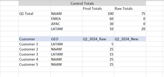
I was given the task to force balance the data in 'Q1_2024_Raw' to sum to the final total by GEO (i.e. all LATAM customers need to sum to 10, so in this case I need to force balance their data down from 20 to 10 and all NAAM customers need to sum to 100 so I need to force balance up from 75 to 100). The results will be placed in 'Q1_2024_New'.

If needed, add percentage change to column J of Control Totals table to adjust based off a percent.

 

[DanteAmor]

Welcome to the MrExcel forum. Please accept my warmest greetings and sincere hope that all is well.

How about:

Dante Amor
	G	H	I	J
1
2			Final Totals	Raw Totals
3	Q1 Total	NAAM	100	75
4		EMEA	60	0
5		APAC	30	0
6		LATAM	10	20
7
8	Customer	GEO	Q1_2024_Raw	Q1_2024_New
9	Customer 1	LATAM	5	2.50
10	Customer 2	NAAM	25	33.33
11	Customer 3	LATAM	15	7.50
12	Customer 4	NAAM	25	33.33
13	Customer 5	NAAM	25	33.33
Hoja4

Cell Formulas
Range	Formula
J9:J13	J9	=I9/VLOOKUP(H9,$H$3:$J$6,3,0)*VLOOKUP(H9,$H$3:$I$6,2,0)

For version 365, the following formula in cell J9 would suffice (based on my example above).

=I9:I13/VLOOKUP(H9:H13,$H$3:$J$6,3,0)*VLOOKUP(H9:H13,$H$3:$I$6,2,0)

----- --
Let me know the result and I'll get back to you as soon as I can.
Sincerely
Dante Amor
----- --

 

[RyanEvert]

Welcome to the MrExcel forum. Please accept my warmest greetings and sincere hope that all is well.

How about:

Dante Amor
	G	H	I	J
1
2			Final Totals	Raw Totals
3	Q1 Total	NAAM	100	75
4		EMEA	60	0
5		APAC	30	0
6		LATAM	10	20
7
8	Customer	GEO	Q1_2024_Raw	Q1_2024_New
9	Customer 1	LATAM	5	2.50
10	Customer 2	NAAM	25	33.33
11	Customer 3	LATAM	15	7.50
12	Customer 4	NAAM	25	33.33
13	Customer 5	NAAM	25	33.33
Hoja4

Cell Formulas
Range	Formula
J9:J13	J9	=I9/VLOOKUP(H9,$H$3:$J$6,3,0)*VLOOKUP(H9,$H$3:$I$6,2,0)

For version 365, the following formula in cell J9 would suffice (based on my example above).

=I9:I13/VLOOKUP(H9:H13,$H$3:$J$6,3,0)*VLOOKUP(H9:H13,$H$3:$I$6,2,0)

----- --
Let me know the result and I'll get back to you as soon as I can.
Sincerely
Dante Amor
----- --

This worked perfectly! Thank you