Hi, I require a formula to work out a sales commission structure as a lot of online templates seem to be different structures.
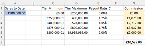
In a nutshell, when looking at the picture, I will require 5 of the same formulas which I can replicate which need to go into the cells in yellow in G2, G3, G4, G5 & G6.
For this basis I will just need the formula for G2 and I can amend it.
The formula will need to take the source value within A2 each time. It will need to tell me the amount of that formula that falls between the lower value C2, and higher value D2. In this case £200,000.00. The same formula then needs to return the percentage of this overall value as shown in E2. As it is 0% it returns £0.
However as you can see within G3 it has returned £1,875.00 which is 1.25% of £149,999.99 (the value below £400,000 and above £250,000.01)
For reference, all values shown within the yellow cells I have inputted myself until I get the formula.
Thanks in advance.