Help needed with a VBA macro which will recognize automatically which data in the named range should be edited

[dangorka]

I have a quite big spreadsheet with several tabs.


The main tab is called "ratings"
There are several named ranges inside the "ratings" tab with same names as names of other tabs in the spreadsheet


This is the photo of the example named range inside ratings tab called "NorTL"

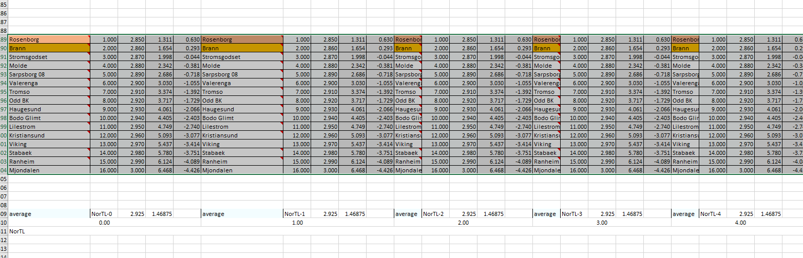
Pls note the numbers outside the range (below "average" from 0 to 4), will move to them now:


This is how tab called "NorTL" looks like

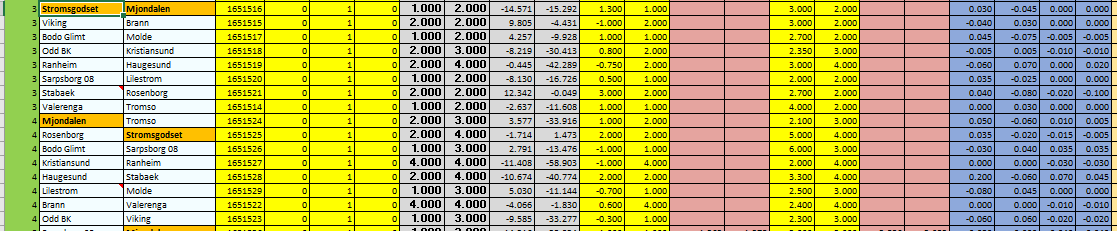
So the key is, to have a macro, which will automatically "apply" values changes listed in blue cells into ratings tab.


For example, if we take first row Stromgodset Mjondalen


Value in column A (green column) = 3 so that means macro has to edit following cells:

Let's call column with numbers from 1 to 16 column A and the next column is column B


Back to the tab with blue cells: first blue cells means adjustment for home team (Stromgodset) which should be applied in column A, second blue cell is adjustment for away team, again applied in column B, third blue cell is an adjustment for home team applied in column B and fourth blue cell is an adjustment for away team which should be added automatically by the macro in column B


So for example from screenshot above, after running macro for this game, updated values should look like this:

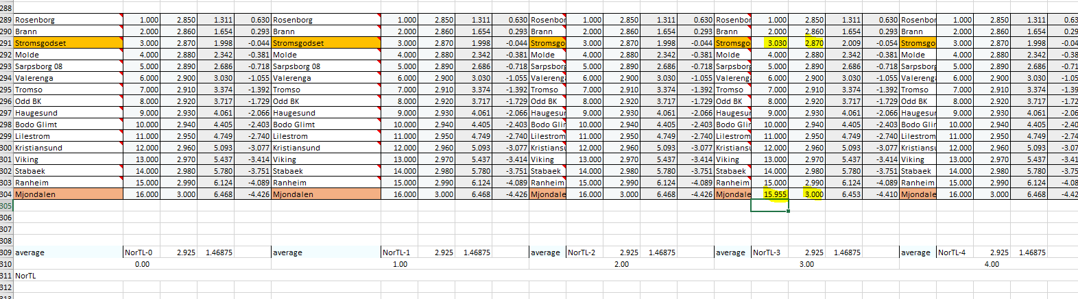
Pls note that for this particular example values in column B are unchanged because values in 3rd and 4th blue cells = 0.00


The biggest challenge here is:


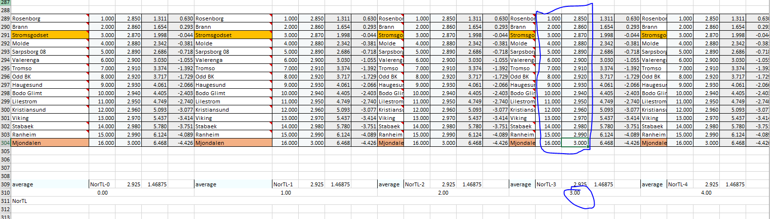
- how to "teach" macro to always find a correct named range inside "ratings" tab
- how to "teach" macro to always find a correct spot inside the named range for applying value changes


Ideally I would like the macro to run numbers update for all games (so for example, if inside the sheet NorTL, in cell B1 there is value "3", macro should run updates for all games which has number "3" added in the first column

 

[dangorka]

"Back to the tab with blue cells: first blue cells means adjustment for home team (Stromgodset) which should be applied in column A, second blue cell is adjustment for away team, again applied in column B, third blue cell is an adjustment for home team applied in column B and fourth blue cell is an adjustment for away team which should be added automatically by the macro in column B"

I made a mistake here, correct text below:

"Back to the tab with blue cells: first blue cells means adjustment for home team (Stromgodset) which should be applied in column A, second blue cell is adjustment for away team, again applied in column A, third blue cell is an adjustment for home team applied in column B and fourth blue cell is an adjustment for away team which should be added automatically by the macro in column B"