How to do Vlookup using VBA to sheet which is filtered?

[dmadhup]

Hi,

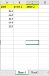
I am doing vlookup to filtered sheet using this code:

Sub test()
Sheets("Sheet1").Select
Range("B2:B6").SpecialCells(xlVisible).FormulaR1C1 = "=VLOOKUP(rc1,Sheet2!c1:c3,2,FALSE)"
End Sub

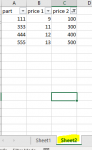
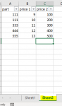
This code works well when sheet1 is filtered. But In my case Sheet2 is filtered not sheet1.

I want to do vlookup from sheet1 (Not filtered) to the sheet2 (filtered). Is there any way I can modify my code to achieve this?

Any help is appreciated.
Thank you!

 

[yky]

Looks to me you just need to swap sheet1 with sheet2 and vice versa and make sure the ranges are correct.

 

[dmadhup]

Looks to me you just need to swap sheet1 with sheet2 and vice versa and make sure the ranges are correct.

Hi,

I know but there is circumstances I can't swap the sheet.

 

[yky]

I meant in the formula, swapping sheets in the formula. I don't see why you can't do it in the formula. Anyway, it'd help if you could post some data.

 

[dmadhup]

I meant in the formula, swapping sheets in the formula. I don't see why you can't do it in the formula. Anyway, it'd help if you could post some data.

Hi,
Below is the attached image of Sheet1 and Sheet2 Data where I want to do vlookup from sheet1 to sheet2 (Filtered)

 

[yky]

What's the expected results?

 

[yky]

It turns out to be more involved than I Thought. Try this:

Sub test()

Range("B2").FormulaArray = "=INDEX(Sheet2!$B$2:$B$6,MATCH(1,IF(SUBTOTAL(3,OFFSET(Sheet2!$B$2:$B$6,ROW($A$2:$A$6)-ROW($A$2),0,1))>0,IF($A$2:$A$6=$A2,1)),0),0)"
Range("B2").Copy Destination:=Range("B3:B6")

End Sub

 

[dmadhup]

It turns out to be more involved than I Thought. Try this:

Sub test()

Range("B2").FormulaArray = "=INDEX(Sheet2!$B$2:$B$6,MATCH(1,IF(SUBTOTAL(3,OFFSET(Sheet2!$B$2:$B$6,ROW($A$2:$A$6)-ROW($A$2),0,1))>0,IF($A$2:$A$6=$A2,1)),0),0)"
Range("B2").Copy Destination:=Range("B3:B6")

End Sub

Hello,

It catches wrong value. For example my sheet2 value is this:

Then I am getting this on sheet1

the price for part 222 should be 1000 not 600.

Thank you!

 

[yky]

When I tested it, it showed #N/A if the corresponding row in sheet2 was filtered off. I got this:

9
#N/A
11
12
13

By the way, my Excel is having problems. I probably need to reinstall Office. Can't test it before reinstalling.

 

[dmadhup]

When I tested it, it showed #N/A if the corresponding row in sheet2 was filtered off. I got this:

9
#N/A
11
12
13

By the way, my Excel is having problems. I probably need to reinstall Office. Can't test it before reinstalling.

Hi,
I see.
But I tested it without applying filter on sheet2. Means if not filtered value is there it suppose to catch it.