If A without B, then C / Employees currently on break based on break list schedule.

Olisthoughts

New Member
Joined
Apr 16, 2020
Messages
33
Office Version
  1. 365
Platform
  1. Windows
Hi,

I'm making a break list at my new job for my team.

Because the list has multiple entries we are forced to concentrate unnecessarily to calculate how many agents are on break. It would be helpful for my colleagues to see how many agents are on break right now, since we have a rule of no more than 3 agents on break at the same time.

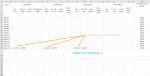
As you'll see in the screenshot, the agents can double-click on a cell for time input under Start time, and double-click on actual return time when they're back.

I'm assuming the way to do it is count the number of agents (rows) that have a value in start time with no value in return time, as that would be an indicator they're on break.

But no matter how I tried I couldn't figure it out. The closest I got was a formula that in pseudo code, basically said If start time + End time equals 1, then 1 agent on break, else nothing. However when more than 1 person was on break it would show 11 instead of 2.

For context, I will attach the codes I'm using (that are working), a screenshot or two, and also, for information, after an agent enters a value in start time or end time, those cells are locked. The estimated return time and actual break time are alway
Screenshot_38.png
Screenshot_38.png
s locked. And there are actually 15 agents on the team, I've only added 4 to work with.

Codes:


Private Sub Worksheet_Change(ByVal Target As Range)

Dim rng As Range
Dim cell As Range

' See if updated cells in watched range
Set rng = Intersect(Target, Range("c:u"))

' Loop through cells in watched range
If Not rng Is Nothing Then
For Each cell In rng
If cell <> "" Then
ActiveSheet.Unprotect Password:="Break"
cell.Locked = True
ActiveSheet.Protect Password:="Break"
End If
Next cell
End If

End Sub

Private Sub Worksheet_BeforeDoubleClick(ByVal Target As Range, Cancel As Boolean)
If Not Intersect(Target, Range("c:u")) Is Nothing Then
Cancel = True
Target.Formula = Time
End If
End Sub
 

Excel Facts

Select a hidden cell
Somehide hide payroll data in column G? Press F5. Type G1. Enter. Look in formula bar while you arrow down through G.
you could do this with a countifs(), but did you want specifically VBA code ?
=COUNTIFS(C:C,"<>"&"",E:E,"") which will give you the count
and then ADD for each range
=COUNTIFS(C:C,"<>"&"",E:E,"") + COUNTIFS(H:H,"<>"&"",J:J,"") + etc
 
Upvote 0
Hello,

Thank you for the response. Since I've never worked with Excel codes and formulas before this, I'm not sure how to make use of your idea.

I tried inputting it into the "agents on break" cell and it just shows me 0.

I can't say I wanted VBA code specifically, but I also wanted the color of the text in the cell to change with each increment. So if 0 agents are on break - open green color, 1 agent - green, 2 agents - yellow, 3 agents - red, 4+ agents - darker red. I assumed this can only be done with code. I only included in this post 1 question, at the advice of a member who helped me with another piece of code.
 

Attachments

  • Screenshot_45.png
    Screenshot_45.png
    36.5 KB · Views: 8
Upvote 0
Is the column E , J O, T
is the cell blank - or a formula present of some kind


In the cell you want the count
and assuming you image is the correct columns
put the formula
=COUNTIFS(C:C,"<>"&"",E:E,"") + COUNTIFS(H:H,"<>"&"",J:J,"") + COUNTIFS(M:M,"<>"&"",O:O,"") + COUNTIFS(R:R,"<>"&"",T:T,"")

If you want the cell with the count in to change colour then you can use conditional formatting
select the cell
GOTO conditional formatting and ADD 4 formula rules

for 2007 or 2010 excel version
Conditional Formatting

Highlight applicable range >>

M20


Home Tab >> Styles >> Conditional Formatting
New Rule >> Use a formula to determine which cells to format
Edit the Rule Description: Format values where this formula is true:


M20 = 1


FormatÖ [Number, Font, Border, Fill] Fill in Green
choose the format you would like to apply when the condition is true
OK >> OK

now repeat for 3 more formula rules

M20 = 2
Fill Yellow

M20 = 3
Fill Red

M20 > = 4
Fill Dark Red
 
Last edited:
Upvote 0
Book2
ABCDEFGHIJKLMNO
1
2startendstartendstartend
3Name 111:0014:00
4Name 213:0012:00
5Name 314:0012:0014:00
6Name 415:00
7
8
94
Sheet1
Cell Formulas
RangeFormula
C9C9=COUNTIFS(C:C,"<>"&"",E:E,"")+COUNTIFS(H:H,"<>"&"",J:J,"")+COUNTIFS(M:M,"<>"&"",O:O,"")
 
Upvote 0
Change the C:C , E:E and other columns to the actual range
C3:C17
for the 15 names
Its because the formula for the count is in a merged cell

Book2
ABCDEFGHIJKLMNOP
1
2startendstartendstartend
3Name 111:0012:0014:0012:00
4Name 213:0012:00
5Name 314:0014:00
6Name 411:00
7Name 5
8Name 6
9Name 7
10Name 8
11Name 9
12Name 10
13Name 11
14Name 12
15Name 13
16Name 14
17Name 15
18
193
Sheet1
Cell Formulas
RangeFormula
C19C19=COUNTIFS(C3:C17,"<>"&"",E3:E17,"")+COUNTIFS(H3:H17,"<>"&"",J3:J17,"")+COUNTIFS(M3:M17,"<>"&"",O3:O17,"")
Cells with Conditional Formatting
CellConditionCell FormatStop If True
C19Expression=C19=3textNO
 
Upvote 0
There must be either something wrong with my work file, or it may interfere with other VBA codes, or formulas, or rules. It's set to lock cells after input.
I tried your formula with a brand new excel file and it works, but it doesn't work in the file with the codes. (It even shows a time instead of a number)
I'll try creating the doc from the beginning, clean, and see what happens.
 
Upvote 0
As I'm recreating the document, is it possible to put text before the formula result, so it doesn't just show a number but for ex. "currently on break:" + formula?
 
Upvote 0
="Currently on Break: " & (COUNTIFS(C:C,"<>"&"",E:E,"") + COUNTIFS(H:H,"<>"&"",J:J,"") + COUNTIFS(M:M,"<>"&"",O:O,"") + COUNTIFS(R:R,"<>"&"",T:T,""))

Book2
ABCDEFGHIJKLMNO
1
2startendstartendstartend
3Name 111:0012:0014:0012:00
4Name 213:0012:00
5Name 314:0014:00
6Name 411:00
7Name 5
8Name 6
9Name 7
10Name 8
11Name 9
12Name 10
13Name 11
14Name 12
15Name 13
16Name 14
17Name 15
18
19Currently on Break: 3
Sheet1
Cell Formulas
RangeFormula
C19C19="Currently on Break: " & (COUNTIFS(C3:C17,"<>"&"",E3:E17,"")+COUNTIFS(H3:H17,"<>"&"",J3:J17,"")+COUNTIFS(M3:M17,"<>"&"",O3:O17,""))
 
Upvote 0
I found that the formula used to count agents on break - can count more agents than there are.

Can it be modified to count the breaks per row somehow, so that in case there are 2 start times without return times on the same row - it would count it as 1, not 2.
 

Attachments

  • Screenshot_52.png
    Screenshot_52.png
    77.1 KB · Views: 9
Upvote 0

Forum statistics

Threads
1,215,521
Messages
6,125,308
Members
449,218
Latest member
Excel Master

We've detected that you are using an adblocker.

We have a great community of people providing Excel help here, but the hosting costs are enormous. You can help keep this site running by allowing ads on MrExcel.com.
Allow Ads at MrExcel

Which adblocker are you using?

Disable AdBlock

Follow these easy steps to disable AdBlock

1)Click on the icon in the browser’s toolbar.
2)Click on the icon in the browser’s toolbar.
2)Click on the "Pause on this site" option.
Go back

Disable AdBlock Plus

Follow these easy steps to disable AdBlock Plus

1)Click on the icon in the browser’s toolbar.
2)Click on the toggle to disable it for "mrexcel.com".
Go back

Disable uBlock Origin

Follow these easy steps to disable uBlock Origin

1)Click on the icon in the browser’s toolbar.
2)Click on the "Power" button.
3)Click on the "Refresh" button.
Go back

Disable uBlock

Follow these easy steps to disable uBlock

1)Click on the icon in the browser’s toolbar.
2)Click on the "Power" button.
3)Click on the "Refresh" button.
Go back
Back
Top