IF Statement with Vlookup including Blank Cell

[Its_All_Dinx]

Hello All

I normal only search the forum for help but no one seems to have answered my burning question.

I would like a Formula but just cannot work out how to do this.

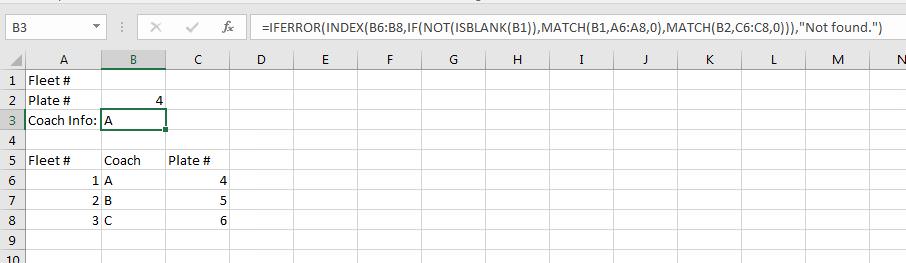
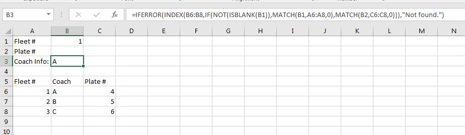
(Small Story) - I have a spread sheet/ data base and I am trying to work out if I put in the fleet number it will tell me some info about the coach, but if the fleet number is blank and I put in the number plate of the coach I want it to return info about the coach

so I need a formula that will look at the first cell for data but if the first cell is blank it will look at the 2nd cell and which ever one has data it will then run the vlookup

If needed I can attached the spread sheet.(not sure how to do this)

This is my currently Formula but it only reads from one cell
=IFERROR(VLOOKUP(B5,'FULL Fleet List'!$A$2:$E$2295,1,FALSE),"No Match Found")

 

[Indystick]

The formula you provided doesn't make sense to me as your lookup value (B5) is inside your table array (A2:E2995). I would think you would be specifying fleet number / plate number outside the table array and returning a result.

Using INDEX/MATCH simplifies this problem greatly, especially since the column you're returning values from is the same in both cases. Assuming your coach info is in the range B2:B2295 (based on your formula):

=IFERROR(INDEX(B6:B8,IF(NOT(ISBLANK(B1)),MATCH(B1,A6:A8,0),MATCH(B2,C6:C8,0))),"Not found.")

I am using NOT(ISBLANK(REF)) to test if the first cell is not empty (you could also just test if it's empty and then reverse the order of the lookups.

This goes on the assumption that Plate Number is column C. Also, I've shifted your table down a few rows to put the lookup cells above.

 

[Its_All_Dinx]

Below is the table I am using

I was just thinking would I be able to use just one cell where I input the fleet number or number plate and it returns all the info below.

At the same time if I enter just the fleet number it shows the number plate and vice versa.

Fleet Number	VRM Number	Location	Tacho fitted	Number of Seats	BUS Type
BYD1472	LJ16EZN	Garage 1	Yes	64	Double Decker
BYD1473	LJ16EZO	Garage 1	yes	64	Double Decker
BYD1474	LJ16EZP	Garage 2	Yes	64	Double Decker
BYD1475	LJ16EZR	Garage 2	yes	64	Double Decker
VWH2115	LK15CXP	Garage 3	Yes	64	Double Decker
VWH2114	LK15CXO	Garage 3	yes	64	Double Decker
VWH2112	LK15CXM	Garage 4	Yes	64	Double Decker
VWH2111	LK15CXL	Garage 4	yes	64	Double Decker
VWH2103	LK15CXB	Garage 5	Yes	64	Double Decker
VWH2093	LK15CWP	Garage 5	yes	64	Double Decker

<tbody>
</tbody>

 

[Indystick]

Either way, the basic principle of the suggested formula remains a valid solution. In the sheet below, I have lookups in D2:G2 to return the data from a row based on either Fleet # or VRM #. The formula is:

=IFERROR(IFNA(INDEX(D6:D15,MATCH($C$2,$C$6:$C$15,0)),INDEX(D6:D15,MATCH($C$2,$B$6:$B$15,0))),"No match.")

Basically it boils down to this: Lookup VRM # (C6:C15) and if there is no match (#N/A), then lookup on Fleet # (D6:D15) and if there is no match for that, return "No match."

In case you're not familiar with INDEX & MATCH, it basically splits up what VLOOKUP/HLOOKUP does into separate components and gives you a lot more flexibility. INDEX is the range of values from which you want to return a value; the first argument of MATCH is your lookup value, the second argument is the lookup array (where you want to find the lookup value), and the match type is 0 (exact) or 1 (<=) or -1 (>=).

 

[Its_All_Dinx]

Hi Indystick

Thank You very much for your help,

I have never used index and match in my life. I had to get my head around this and link it to a spread sheet on a different page.

I will have to experiment and learn the index and match function in more detail

 

[Indystick]

You bet. Pretty much everyone uses INDEX/MATCH once they learn it. There are a couple of reasons it's vastly superior to VLOOKUP / HLOOKUP:

1) Your lookup array (where you're matching) and index array (where you're retrieving) do not have to the same orientation, simply the same array length. For example, your index array could be A1:A5 (a column of values) and your match array could be B1:F1 (a row of values) and it still works.

2) Your lookup array does not need to be in the first column of the table as it does with VLU; nor the top row as it does with HLU.

3) You can do two dimensional lookups (matching on two criteria) where you match on a row and a column and retrieve the value at the intersection.

4) One additional match type - greater than or equal to (not data has to be in descending order for this one to work).

5) Your data doesn't need to be in a table at all. For example, you could have your match array on entirely different worksheet than your index array and it still works.

Learn it! You'll love it!