INDEX MATCH Product code The INDEX in Both Sheets

[Conell8383]

I hope you can help. I have researched a solution but found none that satisfied my problem.
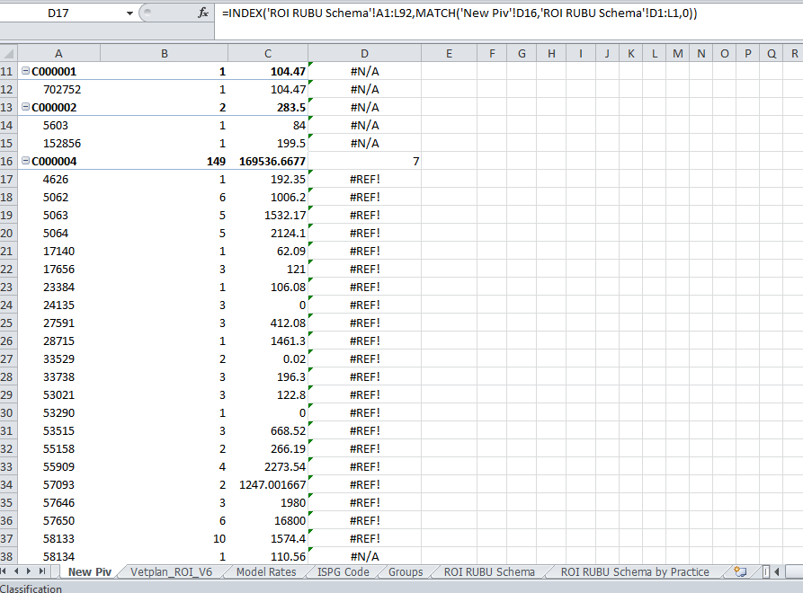
This issue I am facing is this. In Pic 1 you can see that C000004 is my Customer and he has the number 7 in Cell D16. Underneath C000004 you can see more numbers 426, 5062, 5063 etc these are my Product codes on Sheet named New Piv
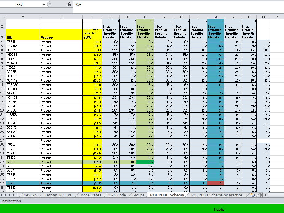
In Pic 2 you can see I am on a new sheet ROI RUBU Schema and in Column A you can see again my Product Codes. Also in Pic 2 you can see from Cells D1 to L1 we have the numbers 1 to 9
Now what I would like to happen is that if a number from Cells D1 to L1 on sheet ROI RUBU Schema is present in Cell D16 New Piv in my example it is 7.
Then I need the formula to recognize Product code 4626 in A17 on sheet New Piv and the product code 4626 in A37 ROI RUBU Schema and that 7 is in J1 on ROI RUBU Schema and that 7 is in D16 on New Piv and return the % value in Cell D17 New Piv
In Pic 2 you can see a colored line showing that I would need 0% returned in Cell D17 in New Piv
Also in Pic 2 you can see another colored line that if the number 3 was present in D17 New Pivproduct code 5062 then I would expect the result in D18 New Piv to be 8%
Essentially what ever number ends up in D16 New Piv I need the percentage vale for the product code from ROI RUBU Schema brought in from ROI RUBU Schema to the product code in New Piv

https://imgur.com/a/R6Mh13R

The formula I have tried is <code style="margin: 0px; padding: 1px 5px; border: 0px; font-style: inherit; font-variant: inherit; font-weight: inherit; font-stretch: inherit; line-height: inherit; font-family: Consolas, Menlo, Monaco, "Lucida Console", "Liberation Mono", "DejaVu Sans Mono", "Bitstream Vera Sans Mono", "Courier New", monospace, sans-serif; font-size: 13px; vertical-align: baseline; box-sizing: inherit; background-color: rgb(239, 240, 241); white-space: pre-wrap;">=INDEX('ROI RUBU Schema'!A1:L92,MATCH('New Piv'!D16,'ROI RUBU Schema'!D1:L1,0))</code>
But I have had no luck. As always any and all help is greatly appreciated.

 

[Conell8383]

Just to Show what the above is Pic 1 is

Pic 2 is

 

[Marcelo Branco]

Maybe...

=INDEX('ROI RUBU Schema'!$D:$L,MATCH(A17,'ROI RUBU Schema'!$A:$A,0),MATCH(D$16,'ROI RUBU Schema'!$D$1:L$1,0))

Not tested, because pictures are not helpful - one cannot copy/paste for testing purposes

M.

 

[Conell8383]

Macrcelo.. You sir!! YOU SIR!! are incredible. I mean Nikola Tesla Next level stuff there. Your formula worked perfectly. Thank you so much for taking the time to respond it is very very much appreciated. Much Respect from Dublin you saved my Irish backside. Have a great day you Genius

 

[Marcelo Branco]

Wow.. thank you very much for your kind words. Much appreciated.

Glad to help

M.