index match question

[monsierexcel]

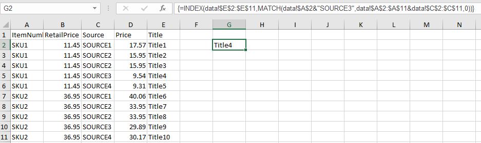
hey all, I have a question about using index/match to return a value

ItemNumber	RetailPrice	Source	Price	Title
SKU1	11.45	SOURCE1	17.57	Title1
SKU1	11.45	SOURCE2	15.95	Title2
SKU1	11.45	SOURCE2	15.95	Title3
SKU1	11.45	SOURCE3	9.54	Title4
SKU1	11.45	SOURCE4	9.31	Title5
SKU2	36.95	SOURCE1	40.06	Title6
SKU2	36.95	SOURCE2	33.95	Title7
SKU2	36.95	SOURCE2	33.95	Title8
SKU2	36.95	SOURCE3	29.89	Title9
SKU2	36.95	SOURCE4	30.17	Title10

<colgroup><col span="5"></colgroup><tbody>
</tbody>

How would i return Title 4 from SKU1 and Source2?
this is in a worksheet called "data"
this is what i have tried so far but cant quite get my head around it!

=INDEX(data!A2:G11,MATCH(A2,A2:A11,0),MATCH(FIND("SOURCE3",data!D:D,1),D2:D11,0))

<tbody>
</tbody>

 

[Fluff]

How about

Excel 2013/2016
	A	B	C	D	E	F	G	H
1	ItemNumber	RetailPrice	Source	Price	Title
2	SKU1	11.45	SOURCE1	17.57	Title1		SKU1	Title4
3	SKU1	11.45	SOURCE2	15.95	Title2		Source3
4	SKU1	11.45	SOURCE2	15.95	Title3
5	SKU1	11.45	SOURCE3	9.54	Title4
6	SKU1	11.45	SOURCE4	9.31	Title5
7	SKU2	36.95	SOURCE1	40.06	Title6
8	SKU2	36.95	SOURCE2	33.95	Title7
9	SKU2	36.95	SOURCE2	33.95	Title8
10	SKU2	36.95	SOURCE3	29.89	Title9
11	SKU2	36.95	SOURCE4	30.17	Title10
Input

Cell Formulas
Range	Formula
H2	{=INDEX(E2:E11,MATCH(G2&"|"&G3,A2:A11&"|"&C2:C11,0))}
Press CTRL+SHIFT+ENTER to enter array formulas.

 

[jkpieterse]

You'll need something like this array formula (entered using control+shift+enter):

=INDEX(data!$G$2:$G$11,MATCH(A2&"|SOURCE2",data!$A$2:$A$11&"|"&data!$C$2:$C$11,0))

 

[6StringJazzer]

It looks like you are searching for a row that has SKU1 as the ItemNumber (you are actually looking at whatever SKU is in row 2, which happens to be SKU1) and SOURCE3 (not Source2, as your description says) as the Source, and return the Title, which in this example is Title4.

I don't understand your column references, because it look like Price is in column D, and title in column E, and you have shown nothing for F and G.

You cannot do that with a simple INDEX/MATCH.

Here is a solution based on your data and description. Note that I have used an array formula. To enter an array formula, once you type the formula, hit CTRL+SHIFT+ENTER (not just ENTER). If you have it correctly you will see {braces} around your formula. You cannot type in the braces, they are just there to indicate an array formula.