Line chart that excludes entries that are "0"

rwilliams09

New Member
Joined
Jun 18, 2017
Messages
48
I am building a template that has the revenue forecast over time and multiple different scenarios will be run through this ONE single template. There are some scenarios where revenue cuts off at 2022 for example and some where it cuts off at 2052. Thus, I have to have the same chart, but since clients will be seeing this chart and altering scenarios, it looks much prettier to only have the line chart show the last year with revenue.

Is there any way to do this? Thanks in advance and Happy Thanksgiving!
 

Excel Facts

Ambidextrous Undo
Undo last command with Ctrl+Z or Alt+Backspace. If you use the Undo icon in the QAT, open the drop-down arrow to undo up to 100 steps.
Re: How to make line chart that excludes entries that are "0"

Thanks! Is there any way to do this without changing the name manager?
 
Upvote 0
Re: How to make line chart that excludes entries that are "0"

Hi,
What I did was modify my formula and worked well for me.
Example
=IF(A1=0,NA(),"your formula")
That did not display the 0 in the graphs.
Hope it works for you.
 
Upvote 0
Re: How to make line chart that excludes entries that are "0"

It removes the 0s from the graph, but I am still stuck with the x-axis (the years) which I would love to not show up at all. The first answer with the name ranges works, but I would like to do it without that or without macros.
 
Upvote 0
Re: How to make line chart that excludes entries that are "0"

You can do this without named formulas and without VBA. You have to have a range of cells for the chart data that is distinct, or separate, from the original data. I've posted an example worksheet you can download at: https://www.dropbox.com/s/7vkyubj997ol3la/dynamic_charts_by_worksheet_formulas.xlsx?dl=0

I used three scenarios:

Alpha scenarioBeta scenarioGamma scenario
AlphaBetaGamma
2017-06-301002017-06-301002017-06-30100
2018-06-30752018-06-301252018-06-30100
2019-06-30502019-06-301502019-06-30100
2020-06-30252020-06-301752020-06-30100
2021-06-3002021-06-302002021-06-30100
2022-06-3002022-06-302252022-06-30100
2023-06-3002023-06-302502023-06-300
2024-06-3002024-06-302752024-06-300

<tbody>
</tbody>

You can select the scenario to graph using a data validation dropdown, cell C5 in my example. The data for the chosen scenario appears in cells B8:C16.

I used a helper cell, M5, to count the non-zero cells in C9:C16, the y-values for the line chart.
=COUNTIF($C$9:$C$16, "<>0")

The first chart uses two multi-cell INDEX+MATCH array formulas to calculate the data to chart. INDEX+MATCH returns #N/A when it fails, and these values won't be plotted on the x-axis. Cells L8:M16 –

Alpha
2017-06-30100
2018-06-3075
2019-06-3050
2020-06-3025
#N/A#N/A
#N/A#N/A
#N/A#N/A
#N/A#N/A

<tbody>
</tbody>

Single multi-cell array formula (Ctrl+Shift+Enter) entered in L9:L16 –
=$B$9:INDEX($B$9:$B$16, $M$5)

Single multi-cell array formula (Ctrl+Shift+Enter) entered in M9:M16 –
=$C$9:INDEX($C$9:$C$16, $M$5)


An alternative is to use IF formulas to determine the points to chart. I show this for the second chart; the data is in cells L25:M32. The helper cell, M5, is used again.

In L25 and copied downward:
=IF(ROW()-ROW($L$24)<=$M$5, B9, NA())

In M25 and copied downward:
=IF(ROW()-ROW($M$24)<=$M$5, C9, NA())


IF formulas and array formulas can cause slow worksheet calculation when used with large data sets. This may or may not be noticeable with your data. The helper cell was used, rather than incorporating the non-zero count formula into the plotted data formulas, to reduce the total number of calculations Excel has to perform.

I used linked cells to change the chart titles as the chosen data set changes.
 
Last edited:
Upvote 0
Re: How to make line chart that excludes entries that are "0"

I am trying this, but for some reason my X-axis is still showing the #N/A and i cant figure out why it is not just excluding it entirely.
 
Upvote 0
Re: How to make line chart that excludes entries that are "0"

Okay i actually have it working now, but the only thing it does NOT do is re-adjust to fill out the entire chart. There is just an empty area where the years and data points no longer exist.
 
Upvote 0
Re: How to make line chart that excludes entries that are "0"

Are you using year numbers only, with no months or days?

The x-axis values should be actual Excel dates formatted to show as years only. Excel treats a line chart with dates on the horizontal axis as a special case of xy-chart.

To leave your original data unchanged (years only), you could change the INDEX+MATCH formula for the charted data years to a date, December 31 in these examples:

=DATE($B$9:INDEX($B$9:$B$16, $M$5), 12, 31)

The similar IF formula would be:

=DATE(IF(ROW()-ROW($L$24)<=$M$5, B9, NA()), 12, 31)

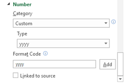
Then use a custom format for the horizontal axis. From the chart format pane:
Format Axis > Axis Options > Axis Options(the column chart icon) > Number.
Select "Custom" in the Category dropdown. In the Format Code box, type "yyyy" then click on the Add button.

5x9UjdG.png
 
Upvote 0

Forum statistics

Threads
1,215,455
Messages
6,124,935
Members
449,195
Latest member
Stevenciu

We've detected that you are using an adblocker.

We have a great community of people providing Excel help here, but the hosting costs are enormous. You can help keep this site running by allowing ads on MrExcel.com.
Allow Ads at MrExcel

Which adblocker are you using?

Disable AdBlock

Follow these easy steps to disable AdBlock

1)Click on the icon in the browser’s toolbar.
2)Click on the icon in the browser’s toolbar.
2)Click on the "Pause on this site" option.
Go back

Disable AdBlock Plus

Follow these easy steps to disable AdBlock Plus

1)Click on the icon in the browser’s toolbar.
2)Click on the toggle to disable it for "mrexcel.com".
Go back

Disable uBlock Origin

Follow these easy steps to disable uBlock Origin

1)Click on the icon in the browser’s toolbar.
2)Click on the "Power" button.
3)Click on the "Refresh" button.
Go back

Disable uBlock

Follow these easy steps to disable uBlock

1)Click on the icon in the browser’s toolbar.
2)Click on the "Power" button.
3)Click on the "Refresh" button.
Go back
Back
Top