I apologise in advance. This issue can seem complicated. However, I'll try to simplify this as much as possible, without leaving out important criteria.
I work in the quality engineering business, and I'll use the relevant terms here:
Supplier number — This is a number that identifies a specific supplier.
Part number — This is a number that identifies a specific part.
Report number — This is a number that identifies a specific report. (A report always contains a supplier, part, and creation date).
What I want, is to lookup a report creation date and report number based on my criteria: Supplier and Part.
Look at the image below. It's divided into three sections: The left is my source data, the middle is what criteria I have, and what I'm missing, and the right is what the solution should look like.
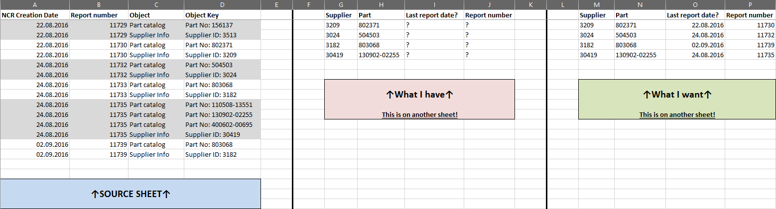
Column B contains the common denominator for the grouping logic. One report number contains 1 supplier and 1 or more parts.
What I want to lookup the report date and number using only the SUPPLIER & PART criteria, as you can see in the middle/right section.
Here's the Excel sheet with this sample for experimentation.
https://drive.google.com/file/d/1q2QrrQQO-gKyd16J_PfiiUiichiOWDWM/view?usp=sharing
Additional info:
This problem would be much simpler if the SOURCE SHEET listed the information such that each row has a unique report value, with a supplier and part value. Such as:
Row 1: Report creation date | Report number | Supplier number | Part number
Row 2: 01.01.2018 11529 3026 805425
Row 3: etcetc...
Then I would just use a INDEX(MATCH(1;(supplier array = supplier)*(part array = part)).
However, here the supplier and part information is scattered on the same column over multiple rows.
EDIT: If anything is unclear feel free to ask.
I work in the quality engineering business, and I'll use the relevant terms here:
Supplier number — This is a number that identifies a specific supplier.
Part number — This is a number that identifies a specific part.
Report number — This is a number that identifies a specific report. (A report always contains a supplier, part, and creation date).
What I want, is to lookup a report creation date and report number based on my criteria: Supplier and Part.
Look at the image below. It's divided into three sections: The left is my source data, the middle is what criteria I have, and what I'm missing, and the right is what the solution should look like.
Column B contains the common denominator for the grouping logic. One report number contains 1 supplier and 1 or more parts.
What I want to lookup the report date and number using only the SUPPLIER & PART criteria, as you can see in the middle/right section.
Here's the Excel sheet with this sample for experimentation.
https://drive.google.com/file/d/1q2QrrQQO-gKyd16J_PfiiUiichiOWDWM/view?usp=sharing
Additional info:
This problem would be much simpler if the SOURCE SHEET listed the information such that each row has a unique report value, with a supplier and part value. Such as:
Row 1: Report creation date | Report number | Supplier number | Part number
Row 2: 01.01.2018 11529 3026 805425
Row 3: etcetc...
Then I would just use a INDEX(MATCH(1;(supplier array = supplier)*(part array = part)).
However, here the supplier and part information is scattered on the same column over multiple rows.
EDIT: If anything is unclear feel free to ask.
Last edited by a moderator:
")


