Match values in ranges

[paata01]

Hi All,
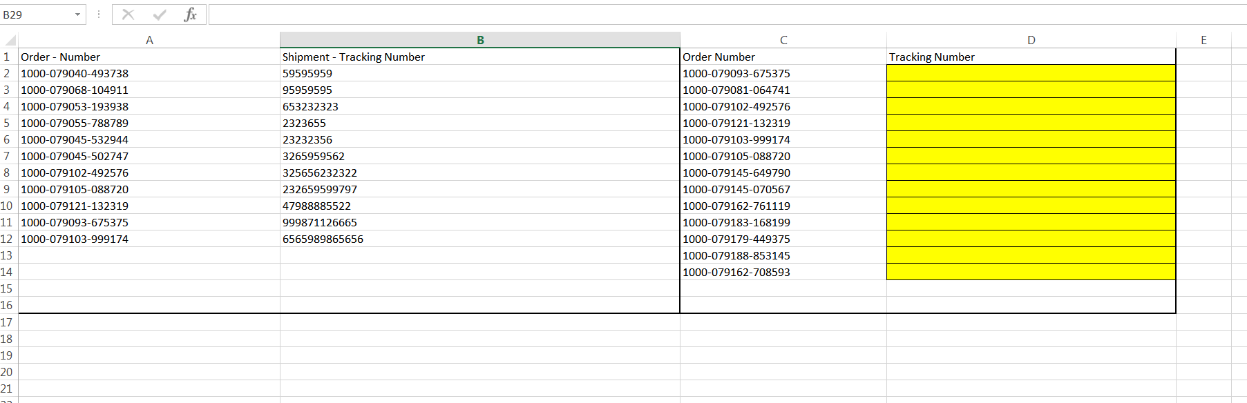
here is what I want to do, I have Orders numbers from customers in column A and tracking numbers in Column B

for example

Order - Number	Shipment - Tracking Number
1000-079031-224355	9400111699000770896629
1000-078438-551504	9400111699000770690593
1000-079019-149952	9400111699000776382126
1000-079003-481137	9400111699000776707851
1000-078980-791552	9400111699000776117261
1000-078991-196564	9400111699000776149316
1000-079003-302571	9400111699000776145462
1000-079001-347526	9400111699000776173557
1000-078991-632512	9400111699000776176176

<colgroup><col><col></colgroup><tbody>
</tbody>

I have another worksheet with same orders numbers but values are not in same raws as first worksheet, I want in second worksheet COLUMN B to copy tracking numbers from Column B from first worksheet and match order numbers, how do I do it with formula. Second worksheet TRACKING NUMBERS Order Number 1000-079081-064741 1000-079145-649790 1000-079145-070567 1000-079162-761119 1000-079183-168199 1000-079179-449375 1000-079188-853145 1000-079162-708593 1000-079197-473195 1000-079210-533389 <colgroup><col></colgroup><tbody> </tbody> something like find similar order number and if match copy from column B here: Thanks!!!!!!!!

<colgroup><col></colgroup><tbody>
</tbody>

 

[Gerald Higgins]

Perhaps using VLOOKUP, such as

=VLOOKUP(C1,A$1:B$100,2,false)

Assumptions:
First value in your second table is in cell C1.
Your original table is in the range A1:B100.

If your data is on two separate tabs, you will need to work the tab references into this formula as appropriate.

 

[paata01]

Perhaps using VLOOKUP, such as

=VLOOKUP(C1,A$1:B$100,2,false)

Assumptions:
First value in your second table is in cell C1.
Your original table is in the range A1:B100.

If your data is on two separate tabs, you will need to work the tab references into this formula as appropriate.

thanks for reply, I tried it but can't do it.

I did this way: in second worksheet TRACKING NUMBER COLUMN (which needs to be populated) =Vlookup(First value of my second table,range of first tables, and what are other values don't really understand it. Thanks again

 

[Gerald Higgins]

Can you post the range for both tables, and also the name of the sheet that contains the first table ?

PS - there is no need to quote my post

 

[C with no eyes]

As G Higgens said, you can use: =VLOOKUP(C1,'name of worksheet 1'!$A:$B,2,false)

To reference a worksheet you need ! at the end of a name. If the worksheet name has spaces you also need to enclose it in ' '

Did you know an easy way to create a formula is simply by clicking the cells or ranges you require?
Here are the steps to creating your formula in B2 assuming your second sheet starts the order numbers in A2 (I have assumed you have a headings in row 1)

Type: =vlookup(,
Click: A1 then sheet1 then A2
Type: ,
Click: sheet2 then entire columns (click and drag over the column headers excel provides e.g. A & B)
Type: 2,false) then hit enter

NB. It will put the reference for columns A:B as sheet2!A:B but you can delete the unnecessary sheet2 reference to make it look tidier.

 

[paata01]

Here is table, I did not really get it how to do. So I want to populate column D with column B tracking numbers for each corresponding order numbers, if it finds same order number copy Tracking number (column B) in column D, if no match leave it blank.
Thank you!

 

[C with no eyes]

You have not provided a table...

We seem to be going in circles.

Order - Number	Shipment - Tracking Number	Order - Number	Shipment - Tracking Number
1000-079031-224355	940011169900071	1000-078438-551504	940011169900072
1000-078438-551504	940011169900072	1000-078980-791552	940011169900075
1000-079019-149952	940011169900073	1000-078991-196564	940011169900076
1000-079003-481137	940011169900074	1000-078991-632512	940011169900079
1000-078980-791552	940011169900075	1000-079001-347526	940011169900078
1000-078991-196564	940011169900076	1000-079003-302571	940011169900077
1000-079003-302571	940011169900077	1000-079003-481137	940011169900074
1000-079001-347526	940011169900078	1000-079019-149952	940011169900073
1000-078991-632512	940011169900079	1000-079031-224355	940011169900071

<tbody>
</tbody>

I had to change the tracking number as excel kept insisting on scientific notation but you get the picture.

I created this in column A to D on a single worksheet. Copy and paste the following into cell D2 then drag it down (using the little black square in the bottom right of the cell when you hover over it)

=VLOOKUP(C2,A:B,2,FALSE)

When you have done this find an order number that you know for certain is not in the first column. It should say #NA . If it does then it's working. To get rid of the error message change the formula in D2 to (and drag it down again)

=IFNA(VLOOKUP(C2,A:B,2,FALSE),"")

If your version of excel will not accept this formula use

=IFERROR(VLOOKUP(C2,A:B,2,FALSE),"")

 

[paata01]

Thank you so much! did it and worked perfectly, I was choosing only A column for second value in formula. =IFNA(VLOOKUP(C2,A:B,2,FALSE),"") works even better leaving blanks instead of errors.
Thanks again ))