Removing invisible characters from VBA array and dynamic formula

[Spencer500]

Hi,

I am building a VBA macro that will run VLOOKUP on user input with the following functionality:

1. Takes in user typed or pasted data from sheet "Main"
2. Ports the data from sheet "Main" to an array.
3. Array processing: Common invisible characters are removed, data is trimmed, data is casted to text to ensure the values to look up and the look-up data set are the same data type to ensure VLOOKUP will work.
4. The array then moves the data to sheet "BlankArray", where a VBA-based dynamic VLOOKUP is run on the data.

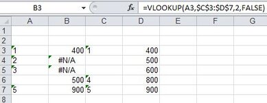
The problem is that invisible characters are somehow being created by this process, which is causing the VLOOKUP to return 500 in cell B6 from cell D4 because a match between A6 and C4 was identified by VLOOKUP. But the respective cells from sheet "Main" from which the data originated are blank.

When I select cell A6, then hit Delete, the invisible character is then deleted, which then causes VLOOKUP to return #NA in cell B6, which is what should happen if the invisible character were not in cell A6.

Invisible characters are also in cells C4 and C5. If I do not delete cell A6, and if I, instead, select C4, then hit delete, VLOOKUP returns 600 in cell B6 from D5 due to the next invisible character match between C5 and A6.

How can I modify this process to remove the invisible characters from appearing in the cells that should be blank? Also, are these invisible characters also appended to the cells that have data? If so, then how can I ensure the invisible characters are not appended to the cells with data? Do you have any other suggestions for improvements?

Please find attached workbook screenshot.

VBA Code:

Public InitialArray As Variant

Sub Match()

Sheets("Main").Select

Dim i As Long
Dim MaxFinalRow As Long


Y1 = 1
Y2 = 1
i = 1

Dim FinalRowValue As Long
Dim FinalRowKey As Long

FinalRowValue = Cells(Rows.Count, 1).End(xlUp).Row

FinalRowKey = Cells(Rows.Count, 3).End(xlUp).Row

FinalRowValueToReturn = Cells(Rows.Count, 4).End(xlUp).Row


If FinalRowValue > FinalRowKey Then
    MaxFinalRow = FinalRowValue
Else
    MaxFinalRow = FinalRowKey
End If


InitialArray = Range(Cells(3, 1), Cells(MaxFinalRow, 4))

Sheets("BlankArray").Select

Range("A1:F13").Select
Selection.ClearContents

    For i = 1 To (FinalRowValue - 2)
        InitialArray(i, 1) = Replace(InitialArray(i, 1), Chr(160), vbNullString)
        InitialArray(i, 1) = Replace(InitialArray(i, 1), Chr(10), vbNullString)
        InitialArray(i, 1) = Replace(InitialArray(i, 1), Chr(13), vbNullString)
        InitialArray(i, 1) = Replace(InitialArray(i, 1), Chr(26), vbNullString)
        InitialArray(i, 1) = Replace(InitialArray(i, 1), Chr(3), vbNullString)
        InitialArray(i, 1) = Replace(InitialArray(i, 1), Chr(28), vbNullString)
    Next i
   
    For i = 1 To (FinalRowKey - 2)
        InitialArray(i, 3) = Replace(InitialArray(i, 3), Chr(160), vbNullString)
        InitialArray(i, 3) = Replace(InitialArray(i, 3), Chr(10), vbNullString)
        InitialArray(i, 3) = Replace(InitialArray(i, 3), Chr(13), vbNullString)
        InitialArray(i, 3) = Replace(InitialArray(i, 3), Chr(26), vbNullString)
        InitialArray(i, 3) = Replace(InitialArray(i, 3), Chr(3), vbNullString)
        InitialArray(i, 3) = Replace(InitialArray(i, 3), Chr(28), vbNullString)
    Next i

    For i = 1 To (FinalRowValue - 2)
        InitialArray(i, 1) = Trim(InitialArray(i, 1))
    Next i
   
    For i = 1 To (FinalRowKey - 2)
        InitialArray(i, 3) = Trim(InitialArray(i, 3))
    Next i


For i = 1 To (FinalRowValue - 2)
    InitialArray(i, 1) = CStr(InitialArray(i, 1))
Next i


For i = 1 To (FinalRowKey - 2)
    InitialArray(i, 3) = CStr(InitialArray(i, 3))
Next i

Range(Cells(3, 1), Cells(MaxFinalRow, 4)) = InitialArray


    Range("B3").Formula = "=VLOOKUP(RC[-1],R3C3:R" & FinalRowKey & "C4,2,FALSE)"
    Range("B3").Select
    Selection.AutoFill Destination:=Range(Cells(3, 2), Cells(FinalRowValue, 2)), Type:=xlFillDefault

End Sub

Thanks.

 

[Alex Blakenburg]

So is it better to run the cast statement before or after the invisible character removal and trim code?

I don't believe your "casting" is serving any purpose. I am not using it my code and I am getting the same results.
If you look in the picture above the 800 is numeric in my sheet main but it has quotes around it in the array in the watch window and is described as a Variant/String.
Regardless of your CStr if you write it out from the Array to a cell formatted General or Number it will convert back to a number.

 

[Spencer500]

Hi Alex,

Your solution results in VLOOKUP to function as expected.

I think this is the best solution because it is array-based.

I did some more testing on this and I think you're right about the array casting step not being necessary. But what appears to continue to be necessary is for columns A and C in the destination sheet to be Text. This ensures that 1 (Number on input sheet) will not be matched with 001 (Text on input sheet).

Thanks.

 

[Alex Blakenburg]

If your numbers aren't numbers that you want to run calculations on but Identification numbers with leading zeroes then you may as well format those columns as text.
You can incorporate that into your code.
You would need to do that "before" you write the data to the sheet.

Columns(1).NumberFormat = "@"
Columns(3).NumberFormat = "@"

 

[Spencer500]

Yes true.

Thanks.