Return Number with -

noraa

New Member
Joined
Mar 16, 2023
Messages
15
Office Version
  1. 2019
Platform
  1. Windows
Hello All,

I need this formula to return a 5 digit number with a - and 2 digits it is matching column A on sheet 2
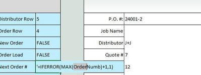
=IFERROR(MAX(OrderNumb)+1,1)


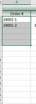
In Column a It reads 24001-1
24001-2
And continues till the end
I would like it to return 24001-3

I have tried formatting both the Cell a column 2 is formatted as ?????-??also tried #####-## no luck.
Any help would be appreciated no VBA please need the formula.
 

Excel Facts

VLOOKUP to Left?
Use =VLOOKUP(A2,CHOOSE({1,2},$Z$1:$Z$99,$Y$1:$Y$99),2,False) to lookup Y values to left of Z values.
Please use XL2BB to post examples of your data and expected results.
 
Upvote 0
Hello,

B6 Sheet1 contains the formula it needs to return the next number sequnce from column A Sheet 2 24001-3. I can only get it to return Number 1 in cell B6 Sheet1
Page 1.JPG
page 2.JPG
 

Attachments

  • Page 1.JPG
    Page 1.JPG
    25.3 KB · Views: 3
  • page 2.JPG
    page 2.JPG
    15.2 KB · Views: 2
Upvote 0
Try

Confirm formula with ctrl+ shift + enter

Book3
ABCDEF
1Order #
224001-1
324001-2
4
5
6Next Order
724001 - 3
824001 - 3
9- 3
10- 3
11- 3
12- 3
13- 3
14- 3
15- 3
16
Sheet1
Cell Formulas
RangeFormula
A7:A15A7=LEFT(C2:C10,SEARCH("-",C2:C10&"-")-1)&" - "&MAX(IFERROR(MID(C2:C10,SEARCH("-",C2:C10&"-")+1,99)+1,0))
Dynamic array formulas.
 
Upvote 0
I've tried changing the formula so that it calls the value from sheet 2 Column A but it keeps giving me a name error.

=LEFT(Sheet2.Range(A3:A10),SEARCH("-",Sheet2.Range(A3:A10)&"-")-1)&" - "&MAX(IFERROR(MID(Sheet2.Range(A3:A10),SEARCH("-",Sheet2.Range(A3:A10)&"-")+1,99)+1,0))

Pretty new to all this. not sure what I am doing wrong or missing?
 
Upvote 0
This is my first Sheet1_ Order. I need cell B6 to increment by 1 number I if there is a blank on Sheet2- Order List Column A3 and increment through Sheet2-Order list column A. Each time an order is addede B6 Will Update to that new order Number plus 1 to the right of the hyphen


1Orderform populate working3-28-2023.xlsm
ABCDE
2Distributor Row5P.O. #:24001-2
3Order Row4Job Name
4New OrderFALSEDistributorJ+J
5Order LoadFALSEQuote #7
6Next Order #=LEFT(Sheet2.Range(A3:A10),SEARCH("-",Sheet2.Range(A3:A10)&"-")-1)&" - "&MAX(IFERROR(MID(Sheet2.Range(A3:A10),SEARCH("-",Sheet2.Range(A3:A10)&"-")+1,99)+1,0))Account #12
Order
Cell Formulas
RangeFormula
B2B2=IFERROR(MATCH(E4,Distributors_Name,0)+2,"")
B3B3=IFERROR(MATCH(E2,OrderNumb,0)+2,"")
Cells with Data Validation
CellAllowCriteria
E4List=Distributors_Name


Since the last number in Sheet 2 A is 24001-2 The next Number that should be in B6 is 24001-3

1Orderform populate working3-28-2023.xlsm
ABCD
1Order List
2Order #DateDistributorAccount #
324001-1
424001-23/28/2023 8:47J+J7
Order List


My Apologies for not using mini sheets earlier it took me a while to figure it out.

Thank you
 
Upvote 0
See if this works

Confirm formula with Ctrl + Shift + Enter

Order Sheet

Book6
ABCDE
1Distributor Row P.O. #:24001-2
2Order Row Job Name
3New OrderFALSEDistributorJ+J
4Order LoadFALSEQuote #7
5Next Order #24001-3Account #12
Order
Cell Formulas
RangeFormula
B1B1=IFERROR(MATCH(E4,Distributors_Name,0)+2,"")
B2B2=IFERROR(MATCH(E2,OrderNumb,0)+2,"")
B5:B12B5=LEFT('Order List'!$A$3:$A$10,SEARCH("-",'Order List'!$A$3:$A$10&"-")-1)&"-"&MAX(IFERROR(MID('Order List'!$A$3:$A$10,SEARCH("-",'Order List'!$A$3:$A$10&"-")+1,99)+1,0))
Dynamic array formulas.


Order List

Book6
ABCD
1Order List
2Order #DateDistributorAccount #
324001-1
424001-245013.37J+J7
Order List
 
Upvote 0
Thank you Sufiyan97,

This formula is returning a -0 which is better than what I was getting but it is not returning a 5 digit incremented # From Column A Sheet 2
 
Upvote 0
Thank you Sufiyan97,

This formula is returning a -0 which is better than what I was getting but it is not returning a 5 digit incremented # From Column A Sheet 2

Have you entered formula with Ctrl + Shift + Enter?


Another Option

Book6
ABCDEF
1Distributor Row P.O. #:24001-2
2Order Row Job Name
3New OrderFALSEDistributorJ+J
4Order LoadFALSEQuote #7
5Next Order #24001-3Account #12
6
7
Order
Cell Formulas
RangeFormula
B1B1=IFERROR(MATCH(E4,Distributors_Name,0)+2,"")
B2B2=IFERROR(MATCH(E2,OrderNumb,0)+2,"")
B5B5=REPLACE(INDEX('Order List'!$A$3:$A$10,COUNTIF('Order List'!$A$3:$A$10,"*")),SEARCH("-",INDEX('Order List'!$A$3:$A$10,COUNTIF('Order List'!$A$3:$A$10,"*")))+1,99,MID(INDEX('Order List'!$A$3:$A$10,COUNTIF('Order List'!$A$3:$A$10,"*")),SEARCH("-",INDEX('Order List'!$A$3:$A$10,COUNTIF('Order List'!$A$3:$A$10,"*")))+1,99)+0+1)
 
Upvote 1
Solution
Thank you Sufiyan97,

Works Great, I was starting to pound my head against the wall. Thank you so much!
 
Upvote 0

Forum statistics

Threads
1,215,491
Messages
6,125,111
Members
449,205
Latest member
ralemanygarcia

We've detected that you are using an adblocker.

We have a great community of people providing Excel help here, but the hosting costs are enormous. You can help keep this site running by allowing ads on MrExcel.com.
Allow Ads at MrExcel

Which adblocker are you using?

Disable AdBlock

Follow these easy steps to disable AdBlock

1)Click on the icon in the browser’s toolbar.
2)Click on the icon in the browser’s toolbar.
2)Click on the "Pause on this site" option.
Go back

Disable AdBlock Plus

Follow these easy steps to disable AdBlock Plus

1)Click on the icon in the browser’s toolbar.
2)Click on the toggle to disable it for "mrexcel.com".
Go back

Disable uBlock Origin

Follow these easy steps to disable uBlock Origin

1)Click on the icon in the browser’s toolbar.
2)Click on the "Power" button.
3)Click on the "Refresh" button.
Go back

Disable uBlock

Follow these easy steps to disable uBlock

1)Click on the icon in the browser’s toolbar.
2)Click on the "Power" button.
3)Click on the "Refresh" button.
Go back
Back
Top