Some advanced Index Match (or something else?)

[Alhelor]

Hello folks,


please take a look at this production table. I need the formulas for A16 and D16:

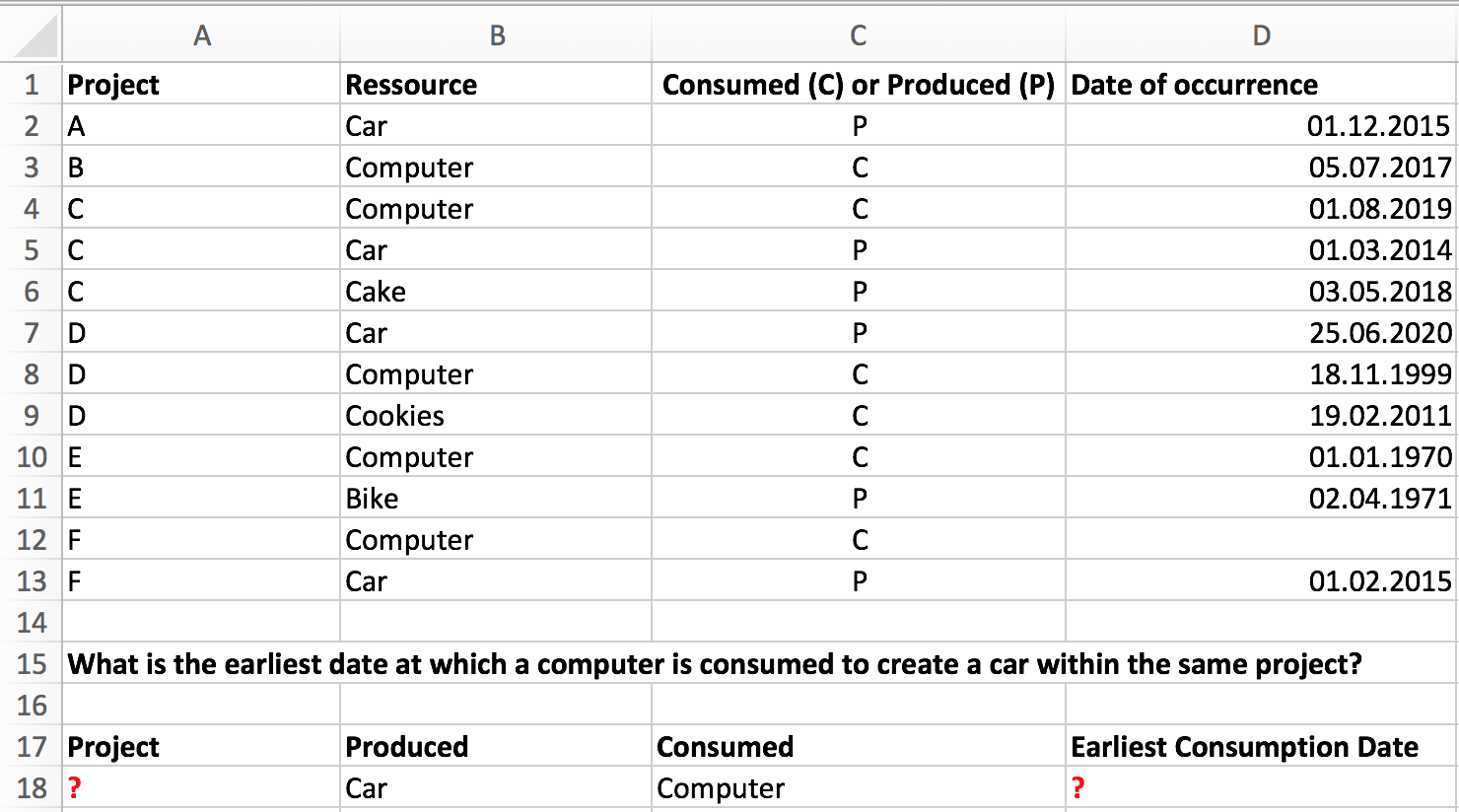
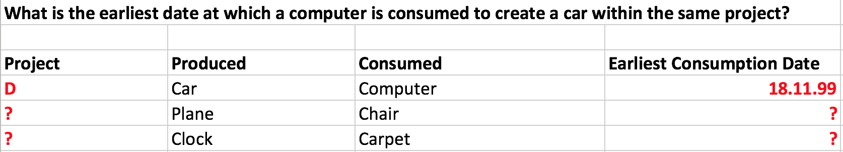
Question: What is the earliest date at which a computer is consumed to create a car within the same project?


A Computer is consumed to produce a Car when they are both part of the same project.


What you can see in the table:


The earliest date at which a Computer is consumed is 01.01.1970. However, it’s project E which doesn’t produce Cars. Projects A and B are independent of each other. Projects C, D and F are the only ones where a Computer is consumed to produce a Car. In project F the relevant date cell is left blank and should be disregarded. In project D, the Computer is consumed earlier than in project C. Thus, D16 should return 18.11.1999 and A16 should return D.


Please help me with the formulas.


Thank you!

P.S.: The fact that in the dates some items are produced before their ingredients are consumed should be disregarded. The production date is not part of this task.

 

[AlanY]

Re: Some advanced Index Match (or something else?) - Please help!

try this

Excel 2012
	A	B	C	D
1
2	P2	Car	C	19/06/2017
3	P3	Car	P	11/05/2017
4	P4		P	13/05/2017
5	P5		C	13/05/2017
6	P6		C	27/03/2017
7	P7	Car	C	02/04/2017
8	P8		C	23/04/2017
9	P9	Car	P	25/05/2017
10	P10	Car	C	01/06/2017
11	P11	Car	P	22/05/2017
12	P12	Car	C	04/06/2017
13	P13		C	07/06/2017
14
15	P7	Car	C	02/04/2017
Sheet1

Cell Formulas
Range	Formula
A15	=INDEX($A$2:$A$13,MATCH(D15,$D$2:$D$13,0))
D15	{=MIN(IF($B$2:$B$13="Car",IF($C$2:$C$13="C",$D$2:$D$13)))}
Press CTRL+SHIFT+ENTER to enter array formulas.

 

[Special-K99]

Re: Some advanced Index Match (or something else?) - Please help!

Homework?

 

[Alhelor]

Re: Some advanced Index Match (or something else?) - Please help!

@AlanY

Thanks for the response. However, that's not the answer. Your formula

1. is looking for a Car being consumed instead of a Computer. But even if you replace that there's a lot of logic missing.
2. doesn't take into account that Computer and Car have to be part of the same project and a Computer needs to be consumed to produce a Car
within that project. Just check out the "What you can see in the Table" part of my post.
3. doesn't ignore blanks in the list of dates.

Nice try though.

 

[Alhelor]

Re: Some advanced Index Match (or something else?) - Please help!

Homework?

I wish. Actual work. Everything is just simplified as much as possible to show the core problem(s) and not bore you with complex production stuff.

 

[AlanY]

Re: Some advanced Index Match (or something else?) - Please help!

you're right, i didn't read your post properly.
have to log off now, hope someone else can chip in

 

[Special-K99]

Re: Some advanced Index Match (or something else?) - Please help!

I think you need a helper column (column F) to identify which projects have cars produced

=INDEX(A$2:A$13,SMALL(IF(($B$2:$B$13="Car")*(C$2:C$13="pP),ROW($A$1:$A$12)),ROW(A1)),1)

This results in rows 1 4 8 and 12 producing projects A C D and F.

Then you need something like

=MIN(IF(AND(B$2:B$13="Computer",C$2:C$13="C",A$2:A$13=F$2:F$13,D$2:D$13<>0),D$2:D$13))
Array formula, use Ctrl-Shift-Enter

to match the Computers consumed and the project letter against the helper column for produced cars
Unfortunately this results in 0 where it should return row 8 project D
But I cant work out why its producing 0.

 

[inactiveuserps07]

Re: Some advanced Index Match (or something else?) - Please help!

@Alhelor, I agree with Special-K99 that use of a helper column makes sense. However, here is a non-array approach:

1. Add Column E formatted as dates, with a header such as "Criteria Matches."

2. In E2, place the following formula and copy down to E13 (in your example):

=IF(AND(B2&C2=$C$18&"C",D2>1000,COUNTIFS(A$2:A$13,A2,B$2:B$13,$B$18,C$2:C$13,"P")>0), D2, "")

3. In D18:

=MIN(E2:E13)

4. In A18:

=INDEX(A$2:A$13,MATCH($D$18,E$2:E$13,0))

However, I'll add that placing your criteria and results (currently in Row 18) directly below what could be a large and growing data set doesn't make sense. If it were me, I'd format the main data set as an official table and use structured references in the above formulas; and I'd move the criteria and results to its own sheet, or at least to the left of the main data table somewhere.

 

[Alhelor]

Re: Some advanced Index Match (or something else?) - Please help!

In reality, this is a huge file with tons of data and of course it's split among different tabs. As I said, this is just an easy version to show the core problem. If it's solved, I'll easily be able to apply it to the big, complex file.

However, Erik, while your solution works, there's a reason I'm looking for a single-cell formula. In reality, it's gonna look somewhat like this:

Thus, I need something I can pull down. The solution with the helper column E only solves it for one example. But the column isn't dynamic, thus, you cannot pull down the formulas from A18 and D18.

Is there another solution or maybe a workaround?

 

[Eric W]

Re: Some advanced Index Match (or something else?) - Please help!

Alhelor: you certainly do like the complicated formulas!

Consider this:

	A	B	C	D	E	F
1	Project	Resource	Consumed © or Produced (P)	Date of occurrence
2	A	Car	P	12/1/2015	0	11/18/1999
3	B	Computer	C	7/5/2017	0
4	C	Computer	C	8/1/2019	0
5	C	Car	P	3/1/2014	0
6	C	Cake	P	5/3/2018	0
7	D	Car	P	6/25/2020	1
8	D	Computer	C	11/18/1999	1
9	D	Cookies	C	2/19/2011	1
10	E	Computer	C	1/1/1970	0
11	E	Bike	P	4/2/1971	0
12	F	Computer	C		0
13	F	Car	P	2/1/2015	0
14
15	What is the earliest date at which a computer is consumed to create a car within the same project?
16
17	Project	Produced	Consumed	Earliest Consumption Date
18	D	Car	Computer	11/18/1999

<colgroup><col style="width: 25pxpx"><col><col><col><col><col><col></colgroup><thead>
</thead><tbody>
</tbody>

Sheet18​

Array Formulas Cell Formula D18 {=SMALL(IF($A$2:$A$13=TRANSPOSE($A$2:$A$13),IF($B$2:$B$13=C18,IF($C$2:$C$13="C",IF(TRANSPOSE($B$2:$B$13)=B18,IF(TRANSPOSE($C$2:$C$13)="P",IF($D$2:$D$13<TRANSPOSE($D$2:$D$13),IF(ISNUMBER($D$2:$D$13),IF(ISNUMBER(TRANSPOSE($D$2:$D$13)),$D$2:$D$13)))))))),1)} A18 {=INDEX($A$2:$A$13,SMALL(IF($D$2:$D$13=D18,IF(COUNTIFS($A$2:$A$13,$A$2:$A$13,$B$2:$B$13,B18,$C$2:$C$13,"P")+COUNTIFS($A$2:$A$13,$A$2:$A$13,$B$2:$B$13,C18,$C$2:$C$13,"C"),ROW($A$2:$A$13)-ROW($A$2)+1)),1))} E2 {=IF(MIN(IF((A2=$A$2:$A$13)*($B$2:$B$13=$C$18)*($C$2:$C$13="C")*ISNUMBER($D$2:$D$13),$D$2:$D$13,2^99))<MAX(IF((A2=$A$2:$A$13)*($B$2:$B$13=$B$18)*($C$2:$C$13="P")*ISNUMBER($D$2:$D$13),$D$2:$D$13,0)),1,0)} F2 {=SMALL(IF((E2:E13=1)*(B2:B13=C18)*(C2:C13="C"),D2:D13),1)} <thead> </thead><tbody> </tbody> Entered with Ctrl+Shift+Enter. If entered correctly, Excel will surround with curly braces {}. Note: Do not try and enter the {} manually yourself

<tbody>
</tbody>

Quite a complicated formula in D18. You can see all of the conditions in it, but when to use TRANSPOSE is a bit hard to explain. The formula in A18 is not guaranteed to find the right project, in case of duplicate dates. But it will only match on projects consuming a computer and producing a car. The requirement for the production date being after the consumed date is not included.

Special-K99 has a point, a helper column might be easier to use. I created a helper column in E2 (which you then drag down), which creates a 1 if the project fulfills all the requirements. Then the shorted formula in F2 gets the date, and the A18 formula would work the same.

Hope this helps!

Edit: Based on a later post I now see, I understand why the helper column may not work for you. Try the D18 formula and let us know.