Sum a set of numbers only up to current month

[cqcqcq]

Hi forum,

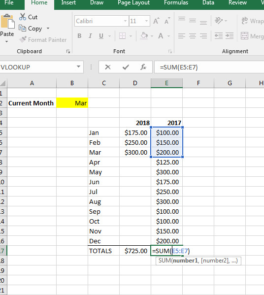
I have a number of sheets that have similar columns with this years total sales and last years sales. On the bottom I'm doing a total, of YTD, but when a month changes, I have to manually go to every last year column and say only sum up to current month.

In other places I am using a dynamic current month name and using sumifs to go grab data for the current month, but I can't figure out how to grab current AND the prior months.

Thanks!

 

[Joe4]

A lot depends on the structure of your data.
Can you post an example of that and your current formulas?

You cannot upload files to this site. But there are tools you can use to post screen images. They are listed in Section B of this link here: http://www.mrexcel.com/forum/board-a...forum-use.html.
Also, there is a Test Here forum on this board that you can use to test out these tools to make sure they are working correctly before using them in your question.

 

[cqcqcq]

Sure!

I have a very dumbed down version of the bigger file ina screenshot below. Essentially the 2017 column has a sum at the bottom. I manually said "Sum Jan - March" what I'd love is for that same formula to start in Jan, but then over to the current month cell (highlighted cell), grab that, and use as it's end part.

 

[Joe4]

I cannot see your image, but my workplace security does block some images for me, so I cannot tell if there really is an image there or not.
It sounds to me like it might just be a matter of updating your formula Can you post it here (since I cannot see the screen print)?

 

[Tyler Hilton]

Hi cqcqcq,

Welcome to the forum! Here is my suggestion:

I would add a helper column in between columns C & D, and within it put the corresponding month number for each month (i.e 1, 2, 3, 4, etc.). Instead of using "Mar" as your current month, use a numerical value 3. Then, in your total rows use a sumifs column with criteria to include months equal to and less than that current month value. Here is an example for the last year total.

=SUMIFS($F$5:$F$16,$D$5:$D$16,"<="&$B$2)

$F$5:$F$16 = sum range
$D$5:$D$16 = criteria range
"<="&$B$2 = criteria value (i.e. less than or equal to current month)

Hope this helps! Shoot me a like if it solves your problem.

Cheers!

Tyler

 

[cqcqcq]

My current formula is insanely rudimentary. =SUM(E5:E7)

To the left of those numbers would be Jan, Feb, Mar and so on... E7 being the March month. Instead, what I want to have happen is I have a separate cell elsewhere which is just using the date function and spitting out the current month as Mar. I want the E7 part of the formula to instead go reference the current month, then look to the left for the corresponding month, and stop summing once it sees that same month.

So this is totally wrong, but like this: =SUM(E5:go look at current month, go look in column B, look for current month and use that as stopping point)

 

[cqcqcq]

Ok interesting, going to have to plug this in and see how it works. Never thought of it this way. I'll give er a try!

Hi cqcqcq,

Welcome to the forum! Here is my suggestion:

I would add a helper column in between columns C & D, and within it put the corresponding month number for each month (i.e 1, 2, 3, 4, etc.). Instead of using "Mar" as your current month, use a numerical value 3. Then, in your total rows use a sumifs column with criteria to include months equal to and less than that current month value. Here is an example for the last year total.

=SUMIFS($F$5:$F$16,$D$5:$D$16,"<="&$B$2)

$F$5:$F$16 = sum range
$D$5:$D$16 = criteria range
"<="&$B$2 = criteria value (i.e. less than or equal to current month)

Hope this helps! Shoot me a like if it solves your problem.

Cheers!

Tyler

 

[Joe4]

Yes, I was going to suggest SUMIFS, if you were not already trying to use it.

If you are always wanting it to be less than or equal to the current month, you can dynamically code that calculation right in the formula.
Modifying Tyler's formula, it would look like this:

[COLOR=#333333]=SUMIFS($F$5:$F$16,$D$5:$D$16,"<=" & [/COLOR][COLOR=#ff0000]EOMONTH(TODAY(),0)[/COLOR][COLOR=#333333])[/COLOR]

 

[cqcqcq]

Thanks so much for the help folks, this is a huge time saver for me.