Taking the right amount out of more than one condition

[JimmyBambo]

Hi friends,
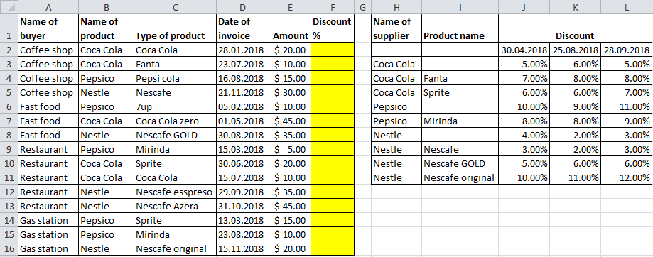
I took picture of my problem as it is easier for me to explain on it, as I cant fully solve this problem.
So I have to determine percentage of discounts (F row) according to conditions in table on right side.
1) For different suppliers I have different discount rates on different dates,
2) For some products of suppliers I have also different discount rates.
So for example, if producer is Coca Cola, product is Coca Cola, date of invoice is 28.01.2018, discount is 5%. If it was product Fanta or Sprite, discount would be 7%.
I hope so that this is solvable, thank you in advance

 

[JimmyBambo]

with this approach you can change both the amounts in the regular discount table

and the discount adjust amounts

eg you could make fred a 0 and make bill a 0.7

<tbody>
</tbody>

Thank you very much for your try and efforts to resolve this problem.
I dont have problem with discount adjustments, because anyways I will put manually these discounts in table (it is big job at the beginning, but that is one-time job).
The problem for me here is that I have more conditions.
As you helped me at the first case, we use helper & helper1, where we said "=Coca Cola&Fanta", and according to that you make OFFSET and everything works fine.

In this case, I have to spread that condition even more.
So we have here for example "Restaurant&Coca Cola&Fanta" (Buyer, Supplier and product) as a helper.
Another problem is that most of the buyers will be in "other buyers", so the formula should recognize buyers from the list, and if they are not listed, than to use discount from "other buyers".
And also, like in previous case, discount is related for the date.
Is it possible to do that with "helper" and OFFSET and "IF ISERROR" for helper1?

 

[oldbrewer]

customer	discountADJUST	product	DISCOUNT	TODAY =	18/12/2018
alan	1.2	pepsi	3.7
alan	1.35	cola	4.85						1	2	3
alan	1.5	nescafe	6						01/10/2018	01/01/2019	01/04/2019
dave	0	pepsi	2.5						31/12/2018	31/03/2019	30/06/2019
ed	0.8	cola	4.3					pepsi	2.5	2.7	2.9
fred	0.6	nescafe	5.1					cola	3.5	3.8	4			MYTABLE
george	0	pepsi	2.5					nescafe	4.5	4.6	4.7
harry	0	cola	3.5											01/01/2018	1
ian	0	nescafe	4.5											31/12/2018	1
														31/03/2019	2
														30/06/2019	3
	NOTE
	alan now has 3 separate discount codes
	for pepsi, cola and nescafe

<colgroup><col><col><col><col><col><col><col span="3"><col span="3"><col span="2"><col><col span="2"></colgroup><tbody>
</tbody>

 

[JimmyBambo]

alan now has 3 separate discount codes

for pepsi, cola and nescafe

<tbody>
</tbody>

I will have 20 main buyers and 1 "other", where I should have all who are not mentioned in this 20 main buyers.
Also I have aprox 250 products at this moment (which can be more in future), so this table will need more than 5000 lines, which could be unreadable.
That is why I am trying to put this buyers in columns, not in rows, and to see is it possible to link it with data which we predefined at the beginning of this problem .

https://www.dropbox.com/s/kvaem9ub8g9mry4/Report (1).xlsx?dl=0

 

[oldbrewer]

buyer	type			TODAY =	18/12/2018
buy1	MAIN
buy99	other
buy2	MAIN
buy3	MAIN
buy70	other
buy71	other
buy72	other
buy73	other
buy74	other
							buyers
							buy1
							buy2
							buy3
							buy4
							buy5
	the main in cell B2 derived by					buy6
							buy7
	=IF(ISERROR(MATCH(A2,$H$17:$H$36,0)),"other","MAIN")		buy8
							buy9
							buy10
							buy11
							buy12
							buy13
							buy14
	so now you only have to maintain the list of main buyers			buy15
							buy16
							buy17
							buy18
							buy19
							buy20

<colgroup><col><col><col><col><col><col><col span="3"></colgroup><tbody>
</tbody>