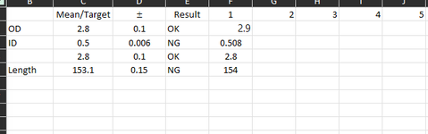
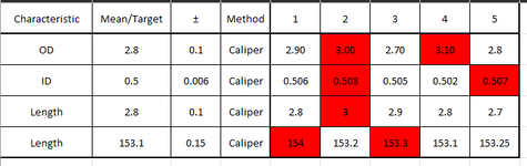
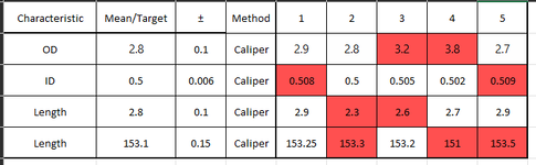
I need a spreadsheet that will show Mean/Target, +/- tolerance but then have the results show Red if out of tolerance. Either text red or cell red. For more than 1 result. Do not need the result "OK" or "NG". Just trying some formulas on that column.
-
If you would like to post, please check out the MrExcel Message Board FAQ and register here. If you forgot your password, you can reset your password.
Tolerance to show out in color
- Thread starter JE79
- Start date
")
Similar threads
- Solved


