Using VBA to copy across columns until a date is reached

[jaspermowatt]

Hello all,

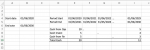
I am trying to create a dynamic cash flow model where I can type in a start and end date, and run the macro, and the the CFM is auto populated i.e. columns are dragged out until the end date is reached.

I have attached an image of a simplified example.

In my head it seems simple, but I am pretty new to the world of macros and I am struggling to make progress. Any help or guidance would be greatly appreciated. Thank you in advance.

J

 

[Yongle]

BEFORE

Book1
	A	B	C	D	E	F	G	H	I	J
2
3
4	Start	01/06/2020		Period start
5				Period end
6	End	31/05/2025
7				CashFrom Ops
8				Cash Invest
9				Cash from fin
10				Total cash	0
11
12				Expenditure1
13				Expenditure2
14				Expenditure3
15				Expenditure4
16				Total spend	0
17
18				Net cash	0
19
Sheet2

Cell Formulas
Range	Formula
E10	E10	=SUM(E7:E9)
E16	E16	=SUM(E12:E15)
E18	E18	=E10-E16

AFTER running CashFlowStructure

Book1
	A	B	C	D	E	F	G	H	I	J
2
3
4	Start	01/06/2020		Period start	01/06/2020	01/06/2021	01/06/2022	01/06/2023	01/06/2024
5				Period end	31/05/2021	31/05/2022	31/05/2023	31/05/2024	31/05/2025
6	End	31/05/2025
7				CashFrom Ops
8				Cash Invest
9				Cash from fin
10				Total cash	0	0	0	0	0
11
12				Expenditure1
13				Expenditure2
14				Expenditure3
15				Expenditure4
16				Total spend	0	0	0	0	0
17
18				Net cash	0	0	0	0	0
19
Sheet2

Cell Formulas
Range	Formula
E10:I10	E10	=SUM(E7:E9)
E16:I16	E16	=SUM(E12:E15)
E18:I18	E18	=E10-E16

Sub CashFlowStructure()
    Dim y As Integer, yrCount As Integer
    Dim startDate As Date, endDate As Date, periodStart As Date, periodEnd As Date
    Dim formulaRng As Range, periodStartCel As Range
    
    Set formulaRng = Range("E7", Range("E" & Rows.Count).End(xlUp))
    Set periodStartCel = Range("E4")
    startDate = Range("B4")
    endDate = Range("B6")
    yrCount = Year(endDate) - Year(startDate)
    
    For y = 1 To yrCount
        periodStart = DateAdd("yyyy", y - 1, startDate)
        periodEnd = DateAdd("yyyy", y, startDate) - 1
    
        With periodStartCel.Offset(, y - 1)
            .Value = periodStart
            .Offset(1).Value = periodEnd
        End With
        formulaRng.Copy formulaRng.Offset(, y - 1)
    Next y
End Sub

You may find this useful

MS Excel: How to use the DATEADD Function (VBA)

This Excel tutorial explains how to use the Excel DATEADD function with syntax and examples. The Microsoft Excel DATEADD function returns a date after which a certain time/date interval has been added.

www.techonthenet.com

 

[jaspermowatt]

Thank you Yongle, appreciate the time you spent writing that up.
It works for the simple situation I used but I am trying to apply to it another scenario, where I am working in quarters. I hoped I could modify your code to suit, but I am still stumped! I have attached a XL2BB, hopefully it works

Reserves and Resources v1.xlsx
	A	B	C	D	E	F	G	H	I	J
1
2		Resources	Tonnes	Grade	Contained		Average Mining Rate per day
3			kt	g/t	koz		Development	10
4		Indicated	8267	3.1	824		Production	30
5		Reserves	Tonnes	Grade	Contained
6			kt	g/t	koz
7		Probable	6942	3.02	674
8		Conversion Rate	84%	97%	82%
9							Q2	Q3	--->>	Qx
10	x	Project Start Date	01 June 2020			Period Start	1-Jun-20	1-Sep-20	--->>	1-Dec-29
11		Construction Duration	20 Months			Period End	31-Aug-20	30-Nov-20	--->>	27-Feb-30
12		Construction End	28 February 2022			Construction	1	1	--->>
13		Production Start	01 March 2022			Production	0	0	--->>
14		Mine Life	8 Years	27 February 2030		End	1	1	--->>
15						Days in Period	91	90	--->>
Sheet8

Cell Formulas
Range	Formula
E4,E7	E4	=C4*K*D4/grm_oz/K
C8:E8	C8	=C7/C4
G9:H9	G9	="Q"&ROUNDUP(MONTH(G10)/3,0)
G10	G10	=C10
H10	H10	=G11+1
G11:H11	G11	=EOMONTH(G10,Month_Quarter-1)
G12:H12	G12	=IF(G11>$C$12,0,1)
G13:H13	G13	=IF(G11<=$C$13,0,1)
G14:H14	G14	=IF($D$14>G10,1,0)
G15:H15	G15	=G11-G10
J10	J10	=J11-88
J11	J11	=D14
C12	C12	=EOMONTH(C10,C11)
C13	C13	=C12+1
D14	D14	=C13+(C14*Day_Year)

Thanks once again.
J

 

[Yongle]

Let's address various items ONE at a time to make sure you do not head down in the wrong direction at this early stage
Everything is 100% your choice and nothing is perfect nor totally straightforward, but it always helps to be aware of a few pitfalls BEFORE jumping in.

Consider cashflow by month
Life is not conveniently split into quarters
Are you absolutely certain that you want the cashflow BUILT by quarter ?
You could BUILD the cashflow by month and then auto-summarise by quarter later
Denominate eveything in months (eg Mine life = 96 months NOT 8 years)

In your example, production is 20 months which is 6 quarters and 2 months
I guarantee that using quarters will create a few numerical headaches for you in quarter 7
One OBVIOUS problem is that the values in rows 12 and 13 need to be BOTH 0 and 1 in quarter 7
- if planning to use those values to drive other calculations change those values to days where they add up to the correct number of days each quarter

Use a formula to do ALL calculations re dates
- the eye does not easily spot date errors and they can be very embarassing and costly!
- there is an error in your example
- construction ends a month earlier than you think ie on 31 January 2022 (= 20 months from 1 June 2020)
- and consequently mining ends a month earlier on 31 January 2030
The formula required in C12
=EDATE(C10,20)-1
I would make C11 NUMERICAL value 20 and then
=EDATE(C10,C11)-1

 

[jaspermowatt]

Thank you again Yongle, and especially thanks for pointing out my errors.

I am still in the early stages but always good to see these errors early.

I've avoided some issues you mention by being limiting the start dates so certain months. For the time being, I'll keep it to quarters but may explore the monthly option later.

Essentially I am now at the stage where I would like to loop through columns, copy and pasting each column and stopping when I get to the end date.

Reserves and Resources v1.xlsx
	A	B	C	D	E	F	G	H	I	J	K	L	M	N	O
1
2		Resources	Tonnes	Grade	Contained
3			kt	g/t	koz
4		Indicated	8267	3.1	824
5		Reserves	Tonnes	Grade	Contained
6			kt	g/t	koz
7		Probable	6942	3.02	674
8		Conversion Rate	84%	97%	82%
9
10	x	Project Start Date	30 June 2020
11		Construction Duration	24 Months
12		Construction End	31 May 2022
13		Production Start	01 June 2022
14		Mine Life	96 Months	31 May 2030
15			8 Years
16		Gold Price	USD/Oz	1250
17		Silver Price	USD/Oz	19.8			Q3	Q4	Q1	Q2	Q3	Q4	Q1	Q2	Q3
18		Gold Recovery	%	91%		Period Start	1-Jul-20	1-Oct-20	1-Jan-21	1-Apr-21	1-Jul-21	1-Oct-21	1-Jan-22	1-Apr-22	1-Jul-22
19		Silver Recovery	%	69.90%		Period End	30-Sep-20	31-Dec-20	31-Mar-21	30-Jun-21	30-Sep-21	31-Dec-21	31-Mar-22	30-Jun-22	30-Sep-22
20		Payable Gold	%	99.80%	PFS pg166	Construction	1	1	1	1	1	1	1	0	0
21		Payable Silver	%	99%	PFS pg166	Production	0	0	0	0	0	0	0	1	1
22		Base Rate Shipment	USD	$ (4,194.00)	PFS pg166	End	1	1	1	1	1	1	1	1	1
23		Frequency of Shipment	Once every:	14 days	PFS pg166	Days in Period	91	91	89	90	91	91	89	90	91
24		Air Freight	USD / kg	$ (5.76)	PFS pg166	Year (Rel. Prod)	-2	-2	-2	-1	-1	-1	-1	1	1
25		Insurance	USD / 1000 USD	$ (0.10)	PFS pg166	Days in Period b4 Prod	-92	-92	-90	-91	-92	-92	-90	0	0
26		Treatment Charge	USD / oz Au	$ (0.75)	PFS pg166
27		State Royalty	%	-3%
28		B2 Royalty	%	-3%
29
30		Mining Cost	USD / t moved	$ (2.46)	PFS pg123+135
31		Processing Cost	USD / t milled	$ (20.46)	PFS pg123+135
32		Tailings	USD / t ore	$ (0.20)	PFS pg123+135
33		G&A	USD / t ore	$ (5.63)	PFS pg123+135
34
35
36
37
38
39
40
41
42
43
44
45
46
47	x	Mining	Units	Source		TOTAL	1-Jul-20	1-Oct-20	1-Jan-21	1-Apr-21	1-Jul-21	1-Oct-21	1-Jan-22	1-Apr-22	1-Jul-22
48		Material Mined	kt	PFS - appendix		101097.00	375	375	375	1433	1433	1433	1433	2208	2208
49		Stripping Ratio	:	PFS - appendix		13.56	0	0	0	148	148	148	148	9	9
50		Ore Mined	kt	PFS - appendix		6942.00	0	0	0	10	10	10	10	212	212
51		Waste Mined	kt	PFS - appendix		94153.00	375	375	375	1423	1423	1423	1423	1996	1996
52		Ore Mined	kt	Calculated		6942.55	0	0	0	9.5928481	9.5928481	9.5928481	9.5928481	212.3076923	212.3076923
53		Waste Mined	kt	Calculated		94154.45	375	375	375	1422.9072	1422.9072	1422.9072	1422.9072	1995.692308	1995.692308
54		Material Mined	kt	Calculated		101097.00	375	375	375	1432.5	1432.5	1432.5	1432.5	2208	2208
55
Sheet1

Cell Formulas
Range	Formula
E4,E7	E4	=C4*K*D4/grm_oz/K
C8:E8	C8	=C7/C4
C12	C12	=EOMONTH(C10,C11-1)
C13	C13	=C12+1
D14	D14	=EOMONTH(C13,C14-1)
C15	C15	=C14/12&" Years"
G17:O17	G17	="Q"&IF(MONTH(G$19)>9,4,IF(MONTH(G$19)>6,3,IF(MONTH(G$19)>3,2,1)))
G18	G18	=C10+1
H18:O18	H18	=G19+1
G19:O19	G19	=EOMONTH(G18,Month_Quarter-1)
G20:O20	G20	=IF(G19>$C$12,0,1)
G21:O21	G21	=IF(G19<=$C$13,0,1)
G22:O22	G22	=IF($D$14>G18,1,0)
G23:O23	G23	=G19-G18
G24:O24	G24	=IF(G20=0,ROUNDUP(SUM($G$21:G21)/Quarter_Year,0),ROUNDUP(SUM(G25:$XFD$25)/Day_Year,0))
G25:O25	G25	=IF(G21=0,G18-H18,0)
G47:O47	G47	=G18
F48,F50:F51	F48	=SUM(G48:XFD48)
G48:O48	G48	=HLOOKUP(G$24,'CFM from PFS'!$S$2:$AD$59,10)
F49	F49	=F51/F50
G49:O49	G49	=HLOOKUP(G$24,'CFM from PFS'!$S$2:$AD$59,6)
G50:O50	G50	=HLOOKUP(G$24,'CFM from PFS'!$S$2:$AD$59,7)
G51:O51	G51	=HLOOKUP(G$24,'CFM from PFS'!$S$2:$AD$59,5)
F52:F54	F52	=SUM(G52:AU52)
G52:O52	G52	=IF(G49>0,G48/(G49+1),0)
G53:O53	G53	=IF(G49=0,G48,G48-(G48/(G49+1)))
G54:O54	G54	=G52+G53

Cells with Conditional Formatting
Cell	Condition		Cell Format	Stop If True
G17:AY114	Expression	=AND(G$20=0,$C$13>=G$18)	text	NO

 

[Yongle]

To copy column G across (as many times as required) it is essential that EVERY formula in every cell in column G works when copied to the next column

One cell that does not work is G18

To work when copied across the formula in G18 it should be replaced with
=F19

AND place this formula in cell F19
=C10+1

AND Use custom number format to display the required text in F19

1. Please confirm that EVERY formula in column G works correctly when pasted manually to column H etc
- if you need nelp making any of the formulas work let me know

2. Do you want the WHOLE column copied across (which is simplest) or something else ?

 

[Yongle]

oops just spotted an error in the above formulas
- I think you can work it out!

 

[Yongle]

I started with this
- note the formulas in EVERY cell to correctly calculated the dates

Book1
	A	B	C	D	E	F	G	H
5
6
7
8
9
10			30/06/2020
11		Construction duration	24 months
12		Construction end	30/06/2022
13		Mine Life	96 months	30/06/2030
14
15
16
17
18						Period Start	01/07/2020
19						Period End	30/09/2020
20
Sheet1

Cell Formulas
Range	Formula
C12	C12	=EDATE(C10,C11)
D13	D13	=EDATE(C12,C13)
G18	G18	=F19+1
F19	F19	=C10
G19	G19	=EDATE(G18,3)-1

The code below copies the WHOLE of column C for the required number of quarters ending in column AT
The dates run as follows
01/07/2020 - 30/09/2020
01/10/2020 - 31/12/2020
01/01/2021 - 31/03/2021
etc
01/04/2030 - 30/06/2030 (column AT)

Sub CopyColumG()
    Dim c As Long, cCount As Long
    For c = 2 To WorksheetFunction.RoundUp((Range("C11") + Range("C13")) / 3, 0)
        Range("G:G").Copy Range("F1").Offset(, c)
    Next c
End Sub

Notes

C11 and C13 both contain a number
Custom format used
0 "months"

F19 gets its value from C10. The formula in F19 is
=C10
Custom format used:
"Period End"

The above should do everything you requested but let me know if it does not

 

[jaspermowatt]

Yongle, that works great, thank you a great deal for your help! Does exactly what I imagined in my head.

All the best,
J

 

[jaspermowatt]

I started with this
- note the formulas in EVERY cell to correctly calculated the dates
The above should do everything you requested but let me know if it does not

I have just added a button (Developer, button) and assigned the macro to it, and it works perfect. However I cannot change the name of the button. I've tried changing its name in the formula tab as google suggested but that didn't work. If you can advice that would be great?

Many thanks,
J