VLOOKUP formula error

[phmalu]

Hi all,

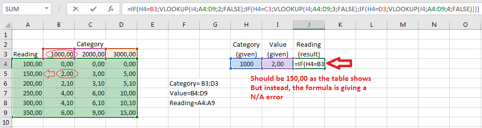
Can you guys try to figure out what's wrong with my formula? Maybe VLOOKUP is not the best function in my case once the desired result will always be in column A but I really don't know what else to try.

=IF(H4=B3;VLOOKUP(I4;A4:D9;2;FALSE);IF(H4=C3;VLOOKUP(I4;A4:D9;3;FALSE);IF(H4=D3;VLOOKUP(I4;A4:D9;4;FALSE))))

Thanks to all!

 

[phmalu]

Very nice, that did solve my problem, thank you so much!

But now I'm having another problem with another data because the column reference and the corresponding values in the table may not match perfectly.
So once I was unsure if it was very or just slightly wrong I've tried to explain what I'm trying to do as well as possible. Hopefully it won't be too confusing.

=INDEX(C3:C9;MATCH(K3;INDEX(D3:G9;0;MATCH(J3;D2:G2;-1));1))

Thank you all once again!!

 

[Aladin Akyurek]

Try...

=INDEX($C$3:$C$9;MATCH(K3;INDEX($D$3:$G$9;0;MATCH(J3;$D$2:$G$2;1)+(LOOKUP(J3;$D$2:$G$2) < J3));1))

 

[phmalu]

Try...

=INDEX($C$3:$C$9;MATCH(K3;INDEX($D$3:$G$9;0;MATCH(J3;$D$2:$G$2;1)+(LOOKUP(J3;$D$2:$G$2) < J3));1))

Apparently that did solve my problem, wow thank you so much!

 

[phmalu]

Apparently that did solve my problem, wow thank you so much!

Nvm, I'm still getting an error when entered value in J3 (for "column") is between 0 and 1. When such value is entered it must pick the largest closest number from the column options which in this case is "1".
But instead, it's giving me the #N/A error again

 

[phmalu]

Nvm, I'm still getting an error when entered value in J3 (for "column") is between 0 and 1. When such value is entered it must pick the largest closest number from the column options which in this case is "1".
But instead, it's giving me the #N/A error again

Just tweaked things a little and figured out that one must assort the array in descending order for the match formula to accept "-1" as the [match_type].
So after finding out that, I changed the data order and then it started calculating things correctly yay
My table does look a little weird but it should do the job for now. But just in case anyone knows how to work-around this formula limitation please let me know. It would be very nice to have the tables in the standard form.

If anyone is wondering, this is how my table and formula look after the tweaks:

=INDEX(C3:C9;MATCH(J3;INDEX(D3:G9;0;MATCH(I3;D2:G2;-1));1))

You may now close this thread

 

[Aladin Akyurek]

What if J3 = 17?

By the way, you could apply the following tweak to the formula which is suggested earlier:

=INDEX($C$3:$C$9,MATCH(K3,INDEX($D$3:$G$9,0,IF(J3 < MIN($D$2:$G$2),MIN($D$2:$G$2),(MATCH(J3,$D$2:$G$2,1)+(LOOKUP(J3,$D$2:$G$2) < J3))),1))):

 

[phmalu]

What if J3 = 17?

By the way, you could apply the following tweak to the formula which is suggested earlier:

=INDEX($C$3:$C$9,MATCH(K3,INDEX($D$3:$G$9,0,IF(J3 < MIN($D$2:$G$2),MIN($D$2:$G$2),(MATCH(J3,$D$2:$G$2,1)+(LOOKUP(J3,$D$2:$G$2) < J3))),1))):

Thank you very much, this new tweak works really good and allows me to use this table assorted in the original format.

Don't worry If the entered value for "column" in J3 is higher than 15 (in this example). I'm currently fixing it with data validation (it must always be between 0 and 15) because those values came from a field experiment. Not amazing but it's getting the job done for now.

However, I believe that something might be hard coded inside your new formula because if I try to use it with a similar table that follows the exact same logic (just with diff. values) it starts misbehaving. I think that happens because in that other tavle the smallest value for "column" (D2:G2) is something higher than 1 (like 2 or 3) then it gives the wrong readings. However, that does not occur with the other formula (=INDEX(C3:C9;MATCH(J3;INDEX(D3:G9;0;MATCH(I3;D2:G2;-1));1) ).That made me think something might be "hard coded" inside the new tweaked formula, otherwise it should work fine just like the other one.
Big thanks again!

 

[Aladin Akyurek]

You are welcome.

We can use indeed a hard coded value instead of MIN($D$2:$G$2).

 

[phmalu]

You are welcome.

We can use indeed a hard coded value instead of MIN($D$2:$G$2).

Original table (calculates correctly):

Modified table w/ minimum value >1 (does not calculate correctly)

Maybe it's easier to understand what I'm trying to say now. I see no reason why your formula is giving wrong readings when the min value for "column" is >1
That made me think something is already hard coded in it and if possible I'd like to change that.
As you can see I'm using the very same formula you provided me earlier but it's not working properly still.
Thank you again!

 

[Aladin Akyurek]

=INDEX($C$3:$C$9,MATCH(K3,INDEX($D$3:$G$9,0,IF(J3 < MIN($D$2:$G$2),1,(MATCH(J3,$D$2:$G$2,1)+(LOOKUP(J3,$D$2:$G$2) < J3)))),1))

Replace comma's with semi-colons for your system.


Note. Please try to post your samples in an Excel readable form as it's tiring to retype what your pictures show.