Add a Calculated Item to Group Items in a Pivot Table

January 26, 2023 - by Bill Jelen

Problem: I’m working with the small data set shown here.

The data set has 7 rows. Product ABC has quantity of 1 and 2. Product DEF has quantity of 4, 8, 16. Product XYZ has quantity of 32 and 64. — Figure 966. The initial data set.

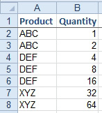
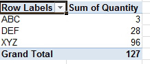
My company has three product lines. The Cocoa Beach plant manufactures ABC and DEF. The Marathon division manufactures XYZ. I have a pivot table that shows sales by product. Remember that the total of items sold is 127.

In the pivot table from the previous data set, the sum of quantity for ABC is 3, for DEF is 28, for XYZ is 96, and the grand total is 127. — Figure 967. You’ve sold 127 units.

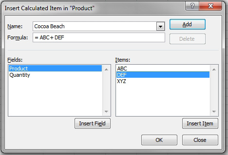
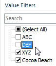
I’ve read that I can add a calculated item along the Product division to total ABC and DEF in order to get a total for the Cocoa Beach plant. I select Insert Calculated Item. In the Insert Calculated Item dialog, I define an item called Cocoa Beach, which is the total of ABC + DEF.

Add a Calculated Item along the product dimension. Your manufacturing plant in Cocoa Beach makes ABC and DEF. The new item, called Cocoa Beach is ABC + DEF. — Figure 968. Add a new item.

However, when I view the resulting pivot table, the total is now wrong. Instead of showing 127 items sold, the pivot table reports that the total is 158.

The pivot table now shows ABC = 3, DEF = 28, XYZ = 96, Cocoa Beach = 31, and the wrong grand total of 158. Any time you create a calculated item, the Grand Total will be wrong. — Figure 969. The total changes from 127 to 158!

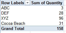
Strategy: Your problem is that the items made in Cocoa Beach are in the list twice, once as ABC and once as Cocoa Beach. The calculated pivot item is a strange concept in Excel. It is one of the least useful items. You should use extreme caution when trying to use a calculated pivot item.

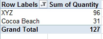
You could use the Product dropdown and uncheck the ABC and DEF items.

One way to "fix" the Grand total is to open the drop-down in A3 and unselect ABC and DEF from the filter. This will leave only XYZ and Cocoa Beach in the pivot table. — Figure 970. The only way to make the total correct is to hide the items used in the calculated item.

The resulting pivot table shows the correct total of 127.

The pivot table now shows XYZ = 96 and Cocoa Beach = 31. The Grand Total is back to the correct value of 127. — Figure 971. Sales are back to 127, but you can’t see the product details.

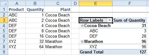
Alternate Strategy: Instead of trying to use a calculated pivot item, you can add a Plant column to the original data. You can then produce a report that shows both the plant location and the products made at the plant, and the total will be correct (127).

Rather than risk having a wrong pivot table due to the calculated item, you could add a Plant column to the original data ABC and DEF are made in Cocoa Beach and XYZ is made in Marathon. In the Pivot Table, put Plant and Product in the Rows and Quantity in Values. The pivot table shows:
Cocoa Beach 31
ABC 3
DEF 28
Marathon 96
XYZ 96
Grand Total 127 — Figure 972. Adding plant info to the original data set solves the problem.

Calculated pivot items sound like they should be useful, but they are not. You should avoid using them.

This article is an excerpt from Power Excel With MrExcel

Title photo by Mel Poole on Unsplash