
Add B5 On All Worksheets
February 01, 2022 - by Bill Jelen

Problem: I have a workbook with 12 monthly sales reports. Each worksheet has identical rows and columns that show sales by week and region. The worksheets are named January, February, …, December. I want to have a Total worksheet that sums cell E5 on all the other worksheets.
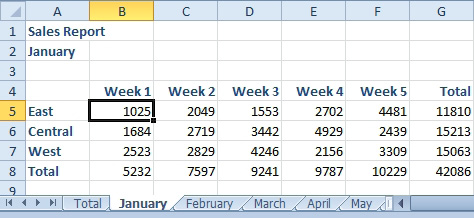
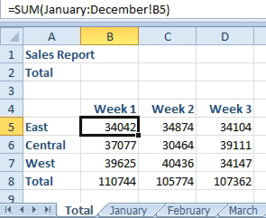
Strategy: You will use a 3D reference to spear through all of the worksheets. In the simplest form, a 3D reference lists the first worksheet, a colon, the second worksheet, an exclamation point, and then the cell address. =SUM(January:December!B5).
Gotcha: The formula is not intelligent. It blindly adds up all of the worksheets that are located between January and December inclusive. If you insert a new worksheet in the middle of this workbook to list your lottery numbers, whatever value is in B5 will get added to the formula shown above. If you would for some reason move the November worksheet to the right of the December worksheet, then the November numbers won’t be included in the formula.
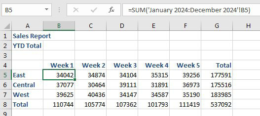
Additional Details: The formula above assumes that you do not have spaces in the worksheet name. If you do have spaces, you will have to add apostrophes around the worksheet names: =SUM(‘January 2014:December 2014!B5).
Additional Details: Here is an easier way to enter this formula:
1. Start in cell B5 on the Total sheet. Type =
SUM(2. Click on the January worksheet. The formula starts as
=SUM(January!3. Shift-Click on the December worksheet. The formula is
=SUM(‘January:December’!4. Click on cell B5. The formula is
=SUM(‘January:December’!B55. Press Enter. The formula changes to
=SUM(January:December!B5)
Thanks to Beth from my seminar at the Louisville Kentucky IMA for the above technique.
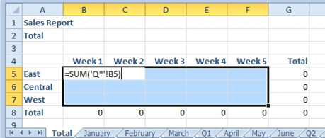
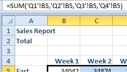
The workbook shown below is fairly amazing. In this workbook, there are already four quarterly worksheets that add up the months from that quarter. You want the Total worksheet to add Q1+Q2+Q3+Q4. In an amazing twist, you can use a wildcard while typing your 3D reference. The wildcard has to be inside apostrophes, even if your worksheet names do not include spaces. Type =SUM(‘Q*!B5). When you accept the formula, Excel will rewrite the formula as =SUM(‘Q1’!B5,’Q2’!B5,’Q3’!B5,’Q4’!B5).
This article is an excerpt from Power Excel With MrExcel
Title photo by Amy Humphries on Unsplash