Add Filter To Selection Functionality

June 11, 2021 - by Bill Jelen

Challenge: Access offers a cool feature called Filter to Selection. If you are looking at a data sheet in Access, click the value XYZ in Field22 and click Filter to Selection, Access shows you only the records where Field22 is equal to XYZ. Excel does not offer this feature. Instead, you have to turn on the Filter (known as AutoFilter in Excel 2003 and before) and choose the desired value from the Filter dropdown.

Solution: It takes only a few lines of code to replicate this feature in VBA. Add the following macros to your Personal Macro Workbook. (To get a Personal Macro Workbook, see “Make a Personal Macro Workbook.”)

Assign the macros to shortcut keys or to custom buttons on your toolbar or Quick Access toolbar in Excel 2007.

Using the First Macro

To use the first macro, in any data set that has a row of headings at the top, select one cell in any column. Click the Filter to Selection icon, as shown in Figure 138.

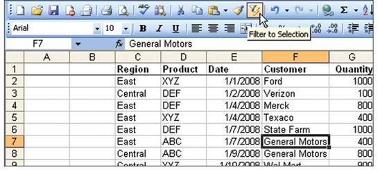
Figure 138. To see all the General Motors records, select one cell that contains General Motors and click Filter to Selection.

Excel hides all the rows that do not contain General Motors in column F (Figure 139).

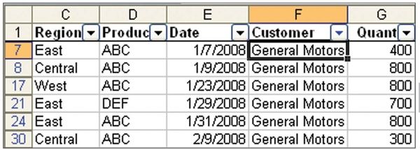
Figure 139. You can filter the data set to show only General Motors records.

Note that the macro is additive: After filtering by customer, you can filter to just ABC records in column D by selecting D8 and clicking Filter to Selection again. You end up with just the sales of ABC to General Motors. Choose the word Central in C8 and click Filter to Selection. You now have just the Central region sales of ABC to General Motors.

To return to all records, you can run the AutoFilterToggle macro or simply turn off the Filter feature. In Excel 2007, you click the large Filter icon on the Data tab. In Excel 2003, you select Data, Filter, Show All or Data, Filter, AutoFilter.

How the Code Works

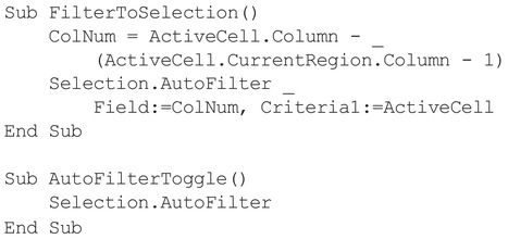
The heart of the code is the line with the AutoFilter method. In this case, the AutoFilter method is applied to the Selection. You are taking advantage of the fact that applying AutoFilter to a single cell automatically applies the filter to the current region. Two named parameters control AutoFilter in this macro. The first parameter is the Field parameter. This is an integer that identifies the column number. In Figure 138, notice that columns A and B are blank. Thus, the current region is C2:H564. The AutoFilter method numbers columns starting with 1 as the leftmost column in the data set. Because column C is the first column in the data set, you specify Field:=1 to filter based on column C.

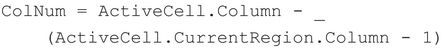
To make the macro more general, you filter to the field number of the active cell. This is stored in a variable called ColNum. You’ll see how ColNum is assigned below.

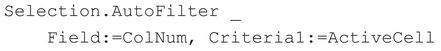
The second parameter for the AutoFilter method is the Criteria1 parameter. To filter the data set to only Exxon customer records, you might use:

Selection.AutoFilter Field:=4, Criteria1:=“Exxon”

The macro specifies a Criteria1 of ActiveCell. The ActiveCell property returns a range object that contains the one cell that is the active cell. Note that someone might select a rectangular range such as C8:H13. Only one of these cells is the active cell. It is the cell listed in the name box. Technically, you should be asking for ActiveCell.Value, but it turns out that the .Value property is the default property returned from a range, so simply filtering to ActiveCell causes Excel to filter to General Motors in Figure 139.

Handling the Unexpected

Most data sets I encounter start in column A. Why would anyone leave columns A and B blank? If you could guarantee that your data sets would always start in column A, then it would be easy to identify the Field parameter as:

If you are in column C, then ActiveCell.Column is 3. Simple enough.

But the macro goes an extra step and envisions someone daring to start a data set in a column other than column A. The logic works sort of like this:

What column is the active cell in? It’s in column F, which is column 6.
Okay. What column is the leftmost column in the data set? It’s in column C, which is 3.
Hmmm. Okay. Then how many blank columns are to the left of the first column? Well, that is the column number of column C minus 1 (i.e., 3 – 1, or 2). In most cases, the calculation for the number of blank columns evaluates to 0. Column A is column number 1, and 1 – 1 is 0.

To translate this logic to VBA, Figure 140 asks many of these questions in the VBA immediate window.

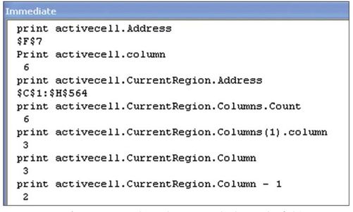
Figure 140. There are some logical steps in calculating the field parameter.

The active cell is F7.

Cell F7 is column number 6.

The current region around F7 is C1:H564. To find the current region, Excel proceeds from the active cell in all directions and stops when it encounters the edge of the spreadsheet or an edge of the data set. An edge of the data set requires the cells in the row below the data set to be completely blank.

When you ask for CurrentRegion.Columns, you are referring to six columns. You might feel compelled to ask for CurrentRegion.Columns (1) .Column to find out that the data set starts in column 3. However, a shortcut is to ask for the Column property of CurrentRegion.Columns. The Column property happens to return the column number of the first column in the range. So, when you ask for CurrentRegion.Column, you get a 3, which indicates that the first column of the current region is in column C.

The first line of the macro goes through all this logic to figure out that Customer is the fourth column in the current data set. ActiveCell.Column is 6. The number of blank columns to the left of the data set is 2. This is ActiveCell. CurrentRegion.Column (3) minus 1. So, the ColNum variable is 6 – 2, or 4.

In order to handle the unexpected, the macro grows to two lines of code. The first line calculates the column number within the current data set:

The second line of code turns on AutoFilter and filters the specific column to the value in the current cell:

Using the Second Macro

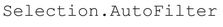
The second macro needs to turn off AutoFilter. If you use the AutoFilter method with no parameters, it simply toggles the AutoFilter dropdown on or off. If a data set is filtered and you use Selection.AutoFilter, Excel turns off AutoFilter and shows all records again. So the second macro is one line of code:

Tip: After this book was written, I learned that this functionality is already in Excel! See the Learn Excel podcast episode 851.

Summary: You can use macros to add the Filter to Selection functionality to Excel.

Title Photo: Joshua Rodriguez on Unsplash

This article is an excerpt from Excel Gurus Gone Wild.