
Array Formulas
September 14, 2017 - by Bill Jelen

Excel Array Formulas are super powerful. You can replace thousands of formulas with a single formula once you learn the Ctrl+Shift+Enter trick. Today, a single array formula does 86,000 calculations.
Triskaidekaphobia is the fear of Friday the 13th. This topic won’t cure anything, but it will show you an absolutely amazing formula that replaces 110,268 formulas. In real life, I never have to count how many Friday the 13ths have occurred in my lifetime, but the power and the beauty of this formula illustrates the power of Excel.
Say that you have a friend who is superstitious about Friday the 13th. You want to illustrate how many Friday the 13ths your friend has lived through.

Set up the simple worksheet below, with birthdate in B1 and =TODAY() in B2. Then a wild formula in B6 evaluates every day that your friend has been alive to figure out how many of those days were Friday and fell on the 13th of the month. For me, the number is 86. Nothing to be afraid of.
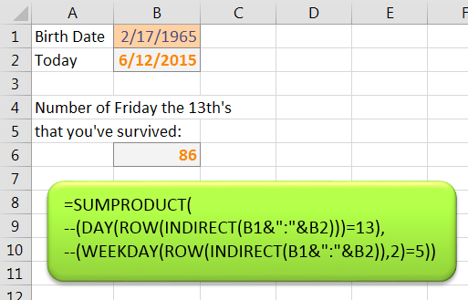
By the way, 2/17/1965 really is my birthday. But I don’t want you to send me a birthday card. Instead, for my birthday, I want you to let me explain how that amazing formula works, one small step at a time.
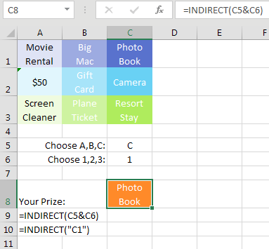
Have you ever used the INDIRECT function? When you ask for =INDIRECT("C3"), Excel will go to C3 and return whatever is in that cell. But INDIRECT is more powerful when you calculate the cell reference on-the-fly. You could set up a prize wheel where someone picks a letter between A and C and then picks a number between 1 and 3. When you concatenate the two answers, you will have a cell address, and whatever is at that cell address is the prize. Looks like I won a photo book instead of the resort stay.
Do you know how Excel stores dates? When Excel shows you 2/17/1965, it is storing 23790 in the cell, because 2/17/1965, was the 23790th day of the 20th century. At the heart of the formula is a concatenation that joins the start date and a colon and the end date. Excel doesn't use the formatted date. Instead, it uses the serial number behind the scenes. So B3&":"&B4 becomes 23790:42167. Believe it or not, that is a valid cell reference. If you wanted to add up everything in rows 3 through 5, you could use =SUM(3:5). So, when you pass 23790:42167 to the INDIRECT function, it points at all of the rows.
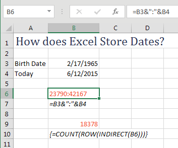
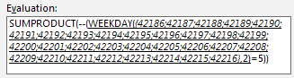
The next thing the killer formula does is to ask for the ROW(23790:42167). Normally, you pass a single cell: =ROW(D17) is 17. But in this case, you are passing thousands of cells. When you ask for ROW(23790:42167) and finish the formula with Ctrl + Shift + Enter, Excel actually returns every number from 23790, 23791, 23792, and so on up to 42167.
This step is the amazing step. In this step, we go from two numbers and “pop out” an array of 18378 numbers. Now, we have to do something with that array of answers. Cell B9 of the previous figure just counts how many answers we get, which is boring, but it proves that ROW(23790:42167) is returning 18378 answers.
Let’s dramatically simplify the original question so you can see what is happening. In this case we'll find the number of Fridays in July 2015. The formula shown below in B7 provides the correct answer in B6.

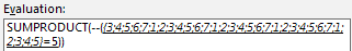
At the heart of the formula is ROW(INDIRECT(B3&":"&B4)). This is going to return the 31 dates in July 2015. But the formula then passes those 31 dates to the WEEKDAY( function. This function will return a 1 for Monday, 5 for Friday, and so on. So the big question is how many of those 31 dates return a 5 when passed to the WEEKDAY(,2) function.
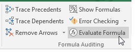
You can watch the formula calculate in slow motion by using the Evaluate Formula command on the Formula tab of the ribbon.
This is after INDIRECT converts the dates to a row reference.
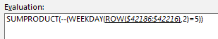
In the next step, Excel is about to pass 31 numbers to the WEEKDAY function. Now, in the killer formula, it would pass 18,378 numbers instead of 31.
Here are the results of the 31 WEEKDAY functions. Remember, we want to count how many are 5.
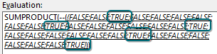
Checking to see if the previous array is 5 returns a whole bunch of True/False values. There are 5 True values, one for each Friday.
I cannot show you what happens next, but I can explain it. Excel cannot SUM a bunch of True and False values. It is against the rules. But if you multiply those True and False values by 1 or if you use the double-negative or the N() function, you convert the True values to 1 and the False values to 0. Send those to SUM or SUMPRODUCT, and you will get the count of the True values.
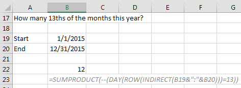
Here is a similar example to count how many months have a day 13 in them. This is trivial to think about: Every month has a 13th, so the answer for a whole year better be 12. Excel is doing the math, generating 365 dates, sending them all to the DAY() function, and figuring out how many end up on the 13th of the month. The answer, as expected, is 12.
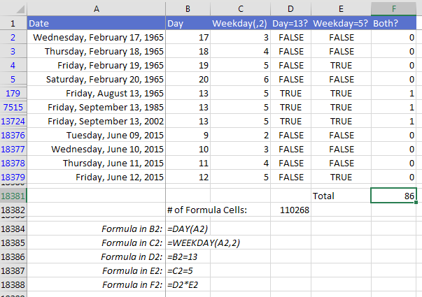
The next figure is a worksheet that does all of the logic the one killer formula shown at the start of this topic. I’ve created a row for every day that I’ve been alive. In column B, I get the DAY() of that date. In column C, I get the WEEKDAY() of the date. In column D, is B equal to 13? In Column E, is C=5? I then multiply D*E to convert the True/False to 1/0.
I’ve hidden a lot of the rows, but I show you three random days in the middle which happen to be both a Friday and the 13th.
The total in F18381 is the same 86 that my original formula returned. A great sign. But this worksheet has 110,268 formulas. My original killer formula does all of the logic of these 110,268 formulas in a single formula.
Wait. I want to clarify. There is nothing magical in the original formula that gets smart and shortens the logic. That original formula really is doing 110,268 steps, probably even more, because the original formula has to calculate the ROW() array twice.
Find a way to use this ROW(INDIRECT(Date:Date)) in real life and send it to me in an e-mail (pub at mrexcel dot com). I’ll send a prize to the first 100 people to answer. Probably not a resort stay. More likely a Big Mac. But that’s the way it goes with prizes. Lots of Big Macs and not many resort stays.
I first saw this formula posted at the MrExcel Message Board in 2003 by Ekim. Credit was given to Harlan Grove. The formula also appeared in Bob Umlas‘s book This Isn't Excel, It's Magic. Mike Delaney, Meni Porat, and Tim Sheets all suggested the minus/minus trick. SUMPRODUCT was suggested by Audrey Lynn and Steven White. Thank you all.
Watch Video
- There are a secret class of formulas called Array Formulas.
- An array formula can do thousands of intermediate calculations.
- They often require you to press Ctrl + Shift + Enter, but not always.
- The best book on array formulas is Mike Girvin's Ctrl + Shift + Enter.
- INDIRECT lets you use concatenation to build something that looks like a cell reference.
- Dates are nicely formatted but are stored as a number of days since January 1 1900.
- Concatenating two dates will point to a range of rows in Excel.
- Asking for the
ROW(INDIRECT(Date1:Date2))will "pop out" an array of many consecutive numbers - Using the WEEKDAY function to figure out if a date is Friday.
- How many Fridays occur in this July?
- To watch a formula calculate in slow motion, use the Evaluate Formula tool
- How many 13ths occur this year?
- How many Friday the 13ths happened between two dates?
- Check each date to see if the WEEKDAY is Friday
- Check each date to see if the DAY is 13
- Multiply those results using SUMPRODUCT
- Use -- to convert True/False to 1/0
Video Transcript
Learn Excel from MrExcel podcast, episode 2026 - My Favorite Formula in All of Excel!
Podcasting this entire book, click the “i” in the top-right hand corner to get to the playlist!
Alright, it was the 30th topic in the book, we were kind of at the end of the formula section, or in the midst of the formula section, and I said I have to include my favorite formula of all time. This is just an amazing formula, whether you have to count the number Friday the 13th or not, it opens a world into a whole secret area of Excel called Array Formulas! Put in a start date, put in an end date, and this formula calculates the number of Friday the 13ths that occurred between those two dates. It's actually doing five calculations on every single day between those two dates, 91895 calculations + SUM, 91896 calculations happening inside of this one little formula, alright. Now, by the end of this episode, you're going to be so intrigued by array formulas. I want to point out, my friend Mike Girvin has the best book on array formulas called “Ctrl+Shift”Enter”, this is a recent printing with the blue cover, used to be a yellow and green cover. Now, whichever one you get, is a great book, same content in both the yellow and the green one.
Alright so, let's start out on the inside of this, with a formula you may not have heard called INDIRECT. INDIRECT allows us to concatenate, or in some way build a bit of text that looks like a cell reference. Alright so, let's say we have a prize wheel here, and I just asked you to choose between A, B, and C. Alright, so you choose this and choose C, and then choose this and choose 3, alright, and your prize is a resort stay, because that's what's stored in C3. And the formula here is concatenated together whatever since C5 and whatever's in C6 using the & and then passing that to the INDIRECT. So =INDIRECT(C5&C6), in this case, is C3, that has to be a balanced out reference. INDIRECT says “Hey, we're going to go to C3 and return the answer from that, alright?” Back in Lotus 1-2-3 this was called the @@function, in Excel they renamed it to be INDIRECT. Alright, so you have in the INDIRECT, now here's the amazing thing that's happening inside of there.
We have two dates, how does Excel store dates, 2/17/1965, that's really just formatting. If we went and looked at the actual number behind that, it is 23790, which means that it is 23790 days since 1/1/1900, and 42167 days since 1/1/1980. On a Mac it'll be since 1/1/1904, so the dates will be about 3000 off. Alright, that's how Excel stores it, it's showing it to us though, thanks to this number format as a date, but if we would concatenate together B3 and a : and B4, it would actually give us the numbers stored behind the scenes. So = B3&”:”&B4, and if we would pass that to INDIRECT, it's actually going to point to all rows from 23790 down to 42167.
So there is the INDIRECT of B6, I asked for the ROW of that, that's going to give me a whole bunch of answers, and to figure out how many answers I used count, alright. And in order to make this work, if I just press Enter, it doesn't work, I have to hold down Ctrl and Shift and press Enter, and see, that adds the {} around the formula up here. It tells Excel to go into super formula mode, array formula mode, and do all of the math for everything popped out from that array, 18378, alright. So, that is an amazing trick, indirect of date1:date2, pass that to the ROW function, and here's a small example.
So we just want to figure out how many Fridays occurred in this July, here's a start date, here's an end date, and for each of those rows I'm going to ask for the WEEKDAY. WEEKDAY tells us what day of the week it is, and here in the ,2 argument Fridays will have a value of 5. So, I'm looking for the answer, and we're going to choose this formula, go to Formulas, and Evaluate Formula, and Evaluate Formula is a great way to watch a formula get calculated in slow motion. So there's the B3, the July 1st, and you see that changes to a number, and then we join the colon, right, there's the B4, that'll change to a number, and now we get the text, 42186:42216. At this point, we pass that to the ROW, and that simple little expression is going to turn into 31 values right here.
Now, in the example where I had everything from 1965 to 2015, it would pop out 86000 values, right, and you don't want to do that and evaluate formula, because would be kind of insane, alright? But you can see what's happening here with the 31, and now I'm passing those 31 days to the WEEKDAY function, and we get 3-4-5. So 3 means that it was a Wednesday, and then 4 means it was a Thursday, and then 5 means it was a Friday. Take all those 31 values and see if they're =5 which is a Friday, and we're going to get a bunch of FALSEs and TRUEs, so Wednesday, Thursday, Friday, and then 7 cells later would be the next TRUE, awesome!
Alright, so in this case we have 5 TRUEs and 26 FALSEs, In order to add those up, I need to convert the FALSE as to 0 and the TRUEs to 1, and a very common way to do that is to use the --. Alright, unfortunately it didn't show the answer there, where we saw a whole bunch of 1’s and 0’s, but that actually is what happens, and then SUMPRODUCT adds it up and gets us to the 5. Down here, if we want to figure out how many of 13th of the month there were this year, from this start date to this end date, very similar process. Although we're going to have 365, pass that to the DAY function, and check to see how many are 13, alright. For the 92000 row example, you know, we're getting the day, we're getting the weekday, checking to see if the, DAY=13, checking to see if the WEEKDAY=FALSE, multiplying this*this, and only in the cases where is a Friday the 13th does that end up as TRUE. The SUMPRODUCT then says “Add all those up”, and that's how we get the 86, literally 91895 calculations + SUM, 91896 happening inside of this one formula, it's crazy powerful! Go buy Mike's book, it's an amazing book, it will open an entire world of Excel formulas to you, and actually, you should just buy both books. Buy my book, buy Mike's book, and you will have an awesome collection that will get you through the rest of the year.
Alright, so recap: there's a secret class of formulas called array formulas, and array formula can do thousands of intermediate calculations. They usually require you to press Ctrl+Shift+Enter, but not always, and the best book on array formulas is Mike Girvin’s “Ctrl+Shift+Enter” book. Alright, so INDIRECT lets you use concatenation to build something that looks like a cell reference, and then INDIRECT goes to that cell reference. Concatenating two dates with a colon will point to a range of rows in Excel, and then asking for the ROW of the INDIRECT of date1:date2 will pop out an array of many consecutive numbers, maybe 31, maybe 365, or maybe 85000. Check each date to see if the WEEKDAY=Friday, check each day to see if the DAY=13, multiply those two arrays of TRUEs and FALSEs using the SUMPRODUCT. In many cases we'll use -- to convert the TRUE/FALSE to 1’s and 0’s to allow the SUMPRODUCT to work. It's an awesome formula, I didn't create it, I found it on the MrExcel message board, as I worked through it, I'm like “Wow, this is really cool!”
Alright, I want to thank you for stopping by, we'll see you next time for another netcast from MrExcel!
Download File
Download the sample file here: Podcast2026.xlsx
Title Photo: GregMontani / Pixabay