Auto-number Records And Columns In An Excel Database

April 09, 2021 - by Bill Jelen

Challenge: You want to build formulas to automatically serially number records and column headers in a database to which AutoFilter is applied and in which selected columns are hidden.

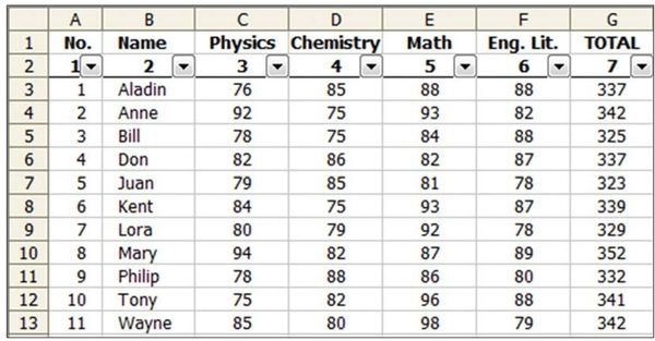
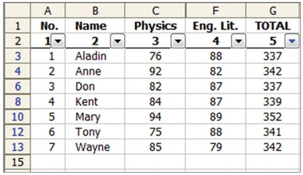
In the database shown in Figures 65 and 66, the records as well as columns are numbered normally. Figure 66 illustrates how the database appears when AutoFilter is applied to show records for total marks > 335 and the columns for Chemistry and Math are hidden. You want to auto-number the records (1 through 7 in this example) and column headers (1 through 5 in this example) by using formulas.

Figure 66. Your goal is to have row labels in A and column labels in row 2 get renumbered as shown here.

Solution: You start by defining the name Database for the range A2:G13. This excludes row 1 from the default selection when you apply AutoFilter. You need to put a space in the first cell immediately following the last record (A14 in this case). (This is a workaround to an annoying Excel bug that shows the last record, regardless of whether it meets the filter criteria.)

In cell A3, enter the formula:

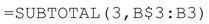
and copy this formula to the range A4:A13.

Notice that the first row reference is absolute and the second one is relative. The formula in A13 is thus:

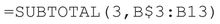
In cell A2, enter the formula:

In cell B2, enter the formula:

and copy it to the range C2:G2.

Notice that the first column reference is absolute and the second one is relative. The formula in G2 is thus:

Now you are set. Breaking It Down: Let’s start with the auto-numbering of the records. The SUBTOTAL function has the syntax SUBTOTAL(type,ref). In your formula, you specified type as 3, which is the equivalent of the COUNTA function. Column B contains names and thus qualifies for use of this subtotal type because the COUNTA function counts the number of text values in a range. The formula makes use of the fact that SUBTOTAL excludes hidden cells from its calculation.

Consider the formula in A10: =SUBTOTAL(3,B$3:B10). The total number of text values in this range is eight, but only five values are visible, so the formula returns 5, which is the serial number you want!

For auto-numbering of the columns, you use the CELL function. The syntax for this function is CELL(info type, [reference]). When you specify “width” as info type, the function returns the column width of the top left cell in reference.

The formula in cell A2, =IF(CELL("width", A1)=0,0,1), returns 0 if column A is hidden and 1 if it is not.

To understand how the formulas in B2:G2 work, first consider the formula in D2:

Because CELL("width", D1) = 0 (column is hidden), the formula evaluates to 0.

The formula in the cell in the next visible column, F2, is:

Because CELL("width",F1)>0, this evaluates to MAX($A2:E2)+1, which is MAX(1,2,3,0,0)+1 = 4.

Gotcha:Although the record numbering auto-updates with changes in AutoFilter settings, the column header numbering does not update as you hide/show columns. You need to force a recalculation by pressing F9 in order for these formulas to update.

Summary: You can build formulas to automatically number records and column headers in a database to which AutoFilter is applied and in which selected columns are hidden.

Title Photo: Siora Photography on Unsplash

This article is an excerpt from Excel Gurus Gone Wild.