
Automatically Number a List of Employees
January 11, 2022 - by Bill Jelen

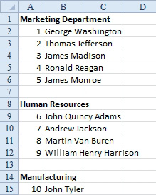
Problem: I work in human resources, and I have a list of employees, separated by department. I have a numeric sequence in column A and the employees’ names in column B. Every time the company hires or fires an employee, I have to manually renumber all the employees. How can I make this job easier?
Strategy: You can replace the numbers in column A with a formula that will count the entries in column B. The formula should count from the current row all the way up to row 1.
The COUNT function will not work because it only counts numeric entries. You need to use the COUNTA function and keep in mind the following points:
- The range that should be counted should extend from B1 to the current row.
- The notation to always use B1 is B$1.
Here’s what you do:
-
1. Enter the formula
=COUNTA(B$1:B2)in cell A2.
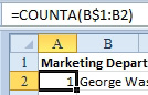
When you copy this formula down a row, the range that is counted will extend from B1 to B3. This is because the B2 portion of the formula is a relative reference that is allowed to change as the formula is copied. The dollar sign in the B$1 reference tells Excel that when you copy the formula, it should always refer to row 1.
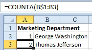
The range now extends from B1 to B3.
2. Copy the formula down to all the names in your list. They will be numbered just as when you typed in the names in manually.
Results: When an employee leaves the company, you can simply delete the row, and all of the later rows will be renumbered. When you hire a new person, you can insert a blank row, enter the new hire’s name, and then copy any formula from another cell in A to the new row.
While this is a specific example, the concept of using a range as an argument where only one portion of the range contains an absolute reference is a common solution to keeping a running total of all cells above the current row.
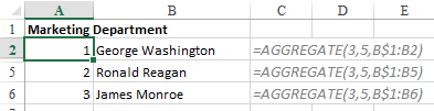
Problem: What if you don’t delete the past employees, but you hide the rows? The newer AGGREGATE function can ignore hidden rows.
In the figure below, the first argument of 3 tells Excel to use the COUNTA function. The second argument of 5 tells Excel to ignore hidden rows.
This article is an excerpt from Power Excel With MrExcel
Title photo by Jeffrey Brandjes on Unsplash